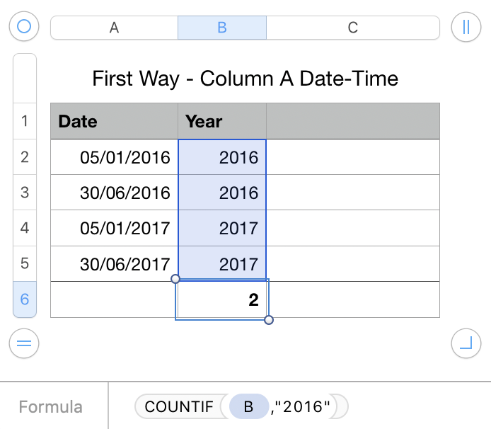
Here are two approaches:

Formula in B2, filled down, is =YEAR(A2)
Formula in B6 (Row 6 defined as Footer Row):
=COUNTIF(B,"2016")

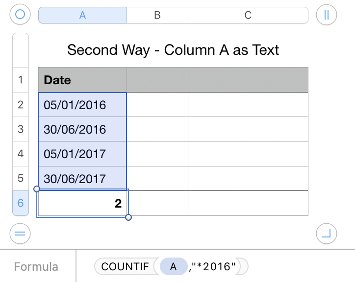
Here the "dates" are entered as text (left-aligned by default).
The formula in A6 (Row 6 is a Footer Row) is:
=COUNTIF(A,"*2016")
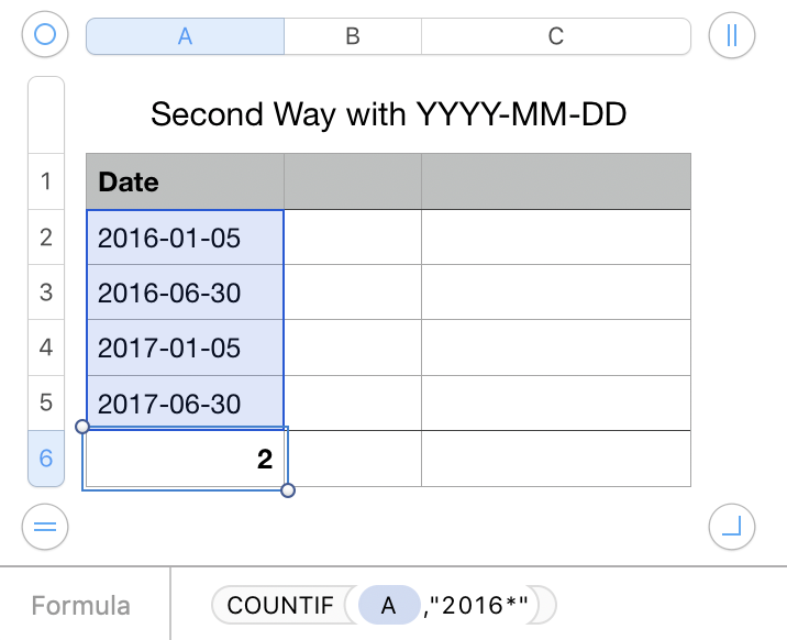
If you use the second approach (entering dates as "text") then the YYYY-MM-DD format works best, as it will sort correctly.
In that case you put the * wildcard after the year in the formula.

=COUNTIF(A,"2016*")
Numbers will happily perform date arithmetic on dates entered as text.
An easy way to tell Number you want to enter as Text is to simply type an apostrophe ( ' ) before the "date". You can also explicitly format the column as Text before making entries.
To convert a column of date-times to text, simply use a formula like this in a new column:
=""&C2
where C2 is the first cell with the right-aligned date-time. Fill that down the column.
Then "remove" the formulas by selecting the new column, typing command-c to copy, and choosing Edit > Paste Formula results.
If you decide to use YYYY-MM-DD because you may want to sort by date, then first change to the format in the Data Format dropdown before converting to Text.
Replace the , in the formulas with ; if your regions uses , as a decimal separator.
SG