Looks like no one’s replied in a while. To start the conversation again, simply ask a new question.

Auto sorting a single column in a Locked table in Numbers

Is there a way to auto sort a column in a locked table? I've created this table and all the cells are populated from results on other sheets. Thus I'm looking to lock this table, so that no mistakes are made by keying over a formula. However, I would also like the last column to somehow auto sort, so that the teams get ranked from highest to lowest automatically. I thought there would be a way to do this through LOOKUP and/or IF statements, but I can't figure out how to do it.


Any help would be greatly appreciated.

iMac with Retina 5K display, macOS 10.15

Posted on May 4, 2020 12:11 PM

Reply
Question marked as Best reply

Posted on May 5, 2020 6:00 PM

Back again.


With the document at the current stage, getting from here to the desired final result is 'most easily' done by transferring data from the 'league' table into a "Leader Board" table containing all or some of the data on the 'league' table ordered descending by the value in the Ranking column


(Air quotes around 'most easily' reflect the frustration of sorting through several syntax and other errors along the way today.)


Top table below is modelled on your League table, with some extra teams added to permit a set of ranks bigger than "1, 2."

I also included two teams with the same "Ranking" score to demonstrate the means of getting the table to list both of these teams, rather than listing one of them twice and the other not at all. Values in the central cells are the same across each row, and show the team's fixed position on the League table list. These values play no part in the sort, which is based solely on the contents of the added column L.


The added column on the League table contains the formula below, entered in L2 and filled down to the end of column L.


L2: K2+ROW(cell)×0.0000001


The formula adds a tiny amount, dependent on the row, to the Rankings value to ensure there will be no duplicates (ties). This makes MATCH find a different value on each search, and INDEX, which uses the number returned by MATCH to determine the row from which to get values for each row in Leader Board.


Leader Board also has one formula, shown below the tables in the image above, entered in A2, filled right to K2, nd filled down to the last row of the table, it collects the data from each cell of League table A2 to the end of column K, maintaining the rank order set in column K (and tweaked to avoid ties in column L).


A2: INDEX(League table::$A:$K, MATCH(LARGE(League table::$L,ROW(cell)−1), League table::$L,0), COLUMN(cell),area-index)


Labels in row 1 are the only manually entered content in Leader Board. Extra rows may be added as needed, and the formulas filled down to those rows.


Regards,

Barry

Similar questions

5 replies
Question marked as Best reply

May 5, 2020 6:00 PM in response to Barry

Back again.


With the document at the current stage, getting from here to the desired final result is 'most easily' done by transferring data from the 'league' table into a "Leader Board" table containing all or some of the data on the 'league' table ordered descending by the value in the Ranking column


(Air quotes around 'most easily' reflect the frustration of sorting through several syntax and other errors along the way today.)


Top table below is modelled on your League table, with some extra teams added to permit a set of ranks bigger than "1, 2."

I also included two teams with the same "Ranking" score to demonstrate the means of getting the table to list both of these teams, rather than listing one of them twice and the other not at all. Values in the central cells are the same across each row, and show the team's fixed position on the League table list. These values play no part in the sort, which is based solely on the contents of the added column L.


The added column on the League table contains the formula below, entered in L2 and filled down to the end of column L.


L2: K2+ROW(cell)×0.0000001


The formula adds a tiny amount, dependent on the row, to the Rankings value to ensure there will be no duplicates (ties). This makes MATCH find a different value on each search, and INDEX, which uses the number returned by MATCH to determine the row from which to get values for each row in Leader Board.


Leader Board also has one formula, shown below the tables in the image above, entered in A2, filled right to K2, nd filled down to the last row of the table, it collects the data from each cell of League table A2 to the end of column K, maintaining the rank order set in column K (and tweaked to avoid ties in column L).


A2: INDEX(League table::$A:$K, MATCH(LARGE(League table::$L,ROW(cell)−1), League table::$L,0), COLUMN(cell),area-index)


Labels in row 1 are the only manually entered content in Leader Board. Extra rows may be added as needed, and the formulas filled down to those rows.


Regards,

Barry

May 5, 2020 3:28 AM in response to Barry

Hi Barry


Yes what you describe is exactly what I am trying to achieve. ie "sort the whole table on the rank values in column K."


MATCH, SMALL & INDEX are entirely new commands to me, but yeah if that is the way to go then it's time I learned how to use them.


Yup I have created separate sheets for each for team. Currently there are only three, but the idea was to create one for any new players that joined us after Lockdown is over as we have a couple of friends that also enjoy the board game.


Below is an example of a team sheet:


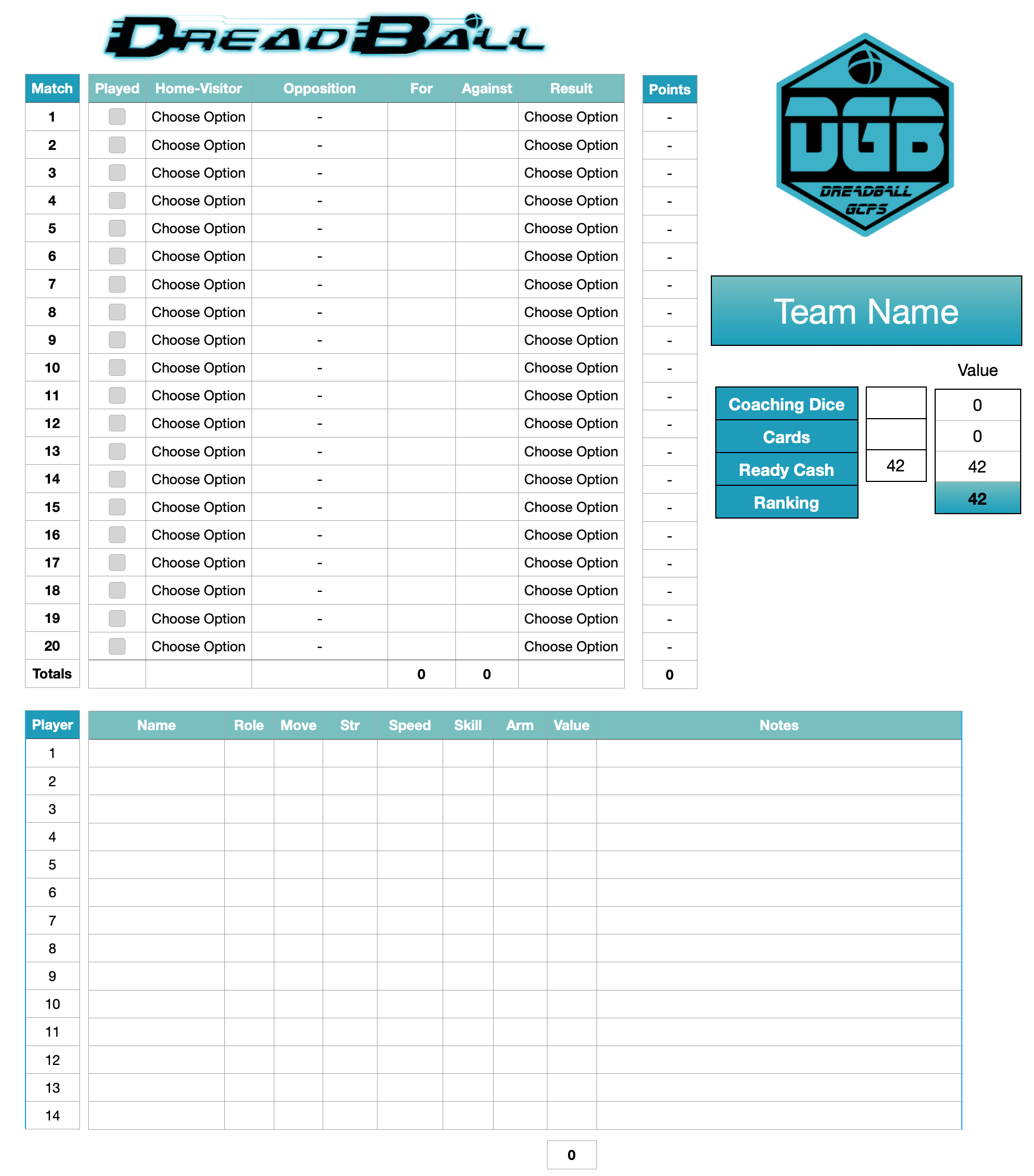
The "Played" column is a simple check box

The "Opposition" column is unformulated and you simply type in the team you played, same goes for the "For" and "Against". columns. You then choose from the drop down box the type of result the score created, ie a 7 - 0 is a Landslide .

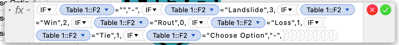
The points are then determined via a series of IF statements as per below


The totals for the "For, Against & Points" Columns are all just simple SUM formulas of the above cells.


Ranking is a simple SUM of the cells above it and the addition of the total value cell that sits below the team roster.


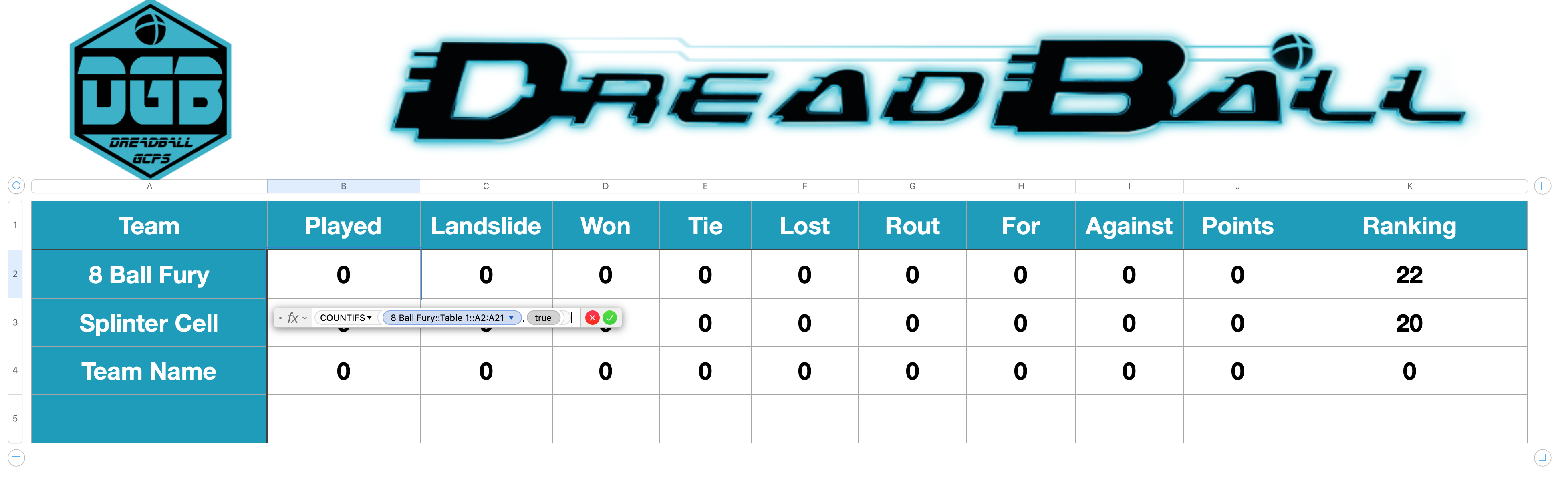
So yeah for each result in the 1st table that I shared (added it again below) the data is pulled from these individual tables on each teams sheet per the above example. I put them together this way, because for this particular board game your team can gain experience, lose players coz they died on the pitch and new players can be bought. Thus I was trying to kill two birds with one stone, by giving each player a sheet that will hold their players attributes and special skills, as well as allowing them to see how they have historically performed against other teams, whilst also giving me the data to create a League table that sorts the teams on overall ranking (higher being better).


So on the league table below for the column "Played" I am using COUNTIFS to draw the data from the relevant teams sheet. Basically I am just counting if the checkbox is ticked for this one.


For the columns "Landslide, Won, Tie, Lost, Rout" I am using COUNTIF in each cell:


for the columns "For, Against, Points & Ranking", I am using the = SUM for each particular cell in the relevant teams sheet.


My plan then hit a brick a wall due my lack of knowledge.


May 5, 2020 12:34 AM in response to Bidge

Hi Bidge, Sorting a single column would not change the order of any other column, including Team Name. If you want the teams listed in rank order, you'll need to sort the whole table on the rank values in column K.


Since the user cannot make changes to a locked table (without unlocking it), you may find it easier to do the calculations on one table, then pull as many columns of the results in rank order using MATCH and SMALL to identify the row containing the current ranks, and INDEX to return the value from the same row of a specified column.


Two teams (or more) with the same rank determining values will be assigned the same rank, and MATCH, given that same rank to look for, will find the same one each time.


To handle this, I usually use an auxiliary column the gets the rank value and adds a tiny amount to that value based on the row on which that team is listed on the original table. My usual value for this is RANK()+ROW()*0.0000001.


Your description above implies that each team has a separate table on which its matches are recorded. If that's the case, pulling the significant data into a single taable might prove complicated.


A more detailed and precise description of your documents valious table would likely be useful.


Regards,

Barry

May 6, 2020 2:37 AM in response to Barry

Thank you so, so, so MUCH. 😁


Took a few tries this morning to get it to work, as I kept getting a syntax error AND I was forgetting to preserve the 1st column in the formula, but I got there through emulating your formula. Much appreciated.


Now I need to go practice it over and over, until I fully understand the process, as its still a bit of copy what you were doing, rather than fully getting it yet.

Auto sorting a single column in a Locked table in Numbers

Welcome to Apple Support Community
A forum where Apple customers help each other with their products. Get started with your Apple ID.