Hide zero's in Numbers 10.0

Rob99fla wrote:

How do I hide zero values as you can in Excel?

Numbers has custom formats very similar to Excel. To hide zeros the way you would in Excel, without changing the underlying formulas, you can select the cells and in the Cell tab of the inspector at the right go to the Data Format dropdown and choose "Custom Format"

Click 'Add a rule' and set it up like this:

Result:

SG

Hi Rob,

Calculating 'Units Added' in column F, using a subset of your table. My Language and Region settings show GBP (Great British Pound).

Copy this formula and paste into F3 =IF(E3÷G3>0,E3÷G3,"")

Or you can type into F3 =IF(E3/G3>0,E3/G3,"") and Numbers will change slash (/) to the division symbol (÷).

Fill the formula down column F

In English, if the result of the formula is greater than zero, then return the result of the formula.

Else (the result is not greater than zero), return "" (the NULL character).

BTW, you can show the table name. Click on the table and Format Panel (on the right) > Table tab > Tick Table Name

Then, if you like, you can delete row 1 of the table. Formulas will automatically adjust.

Regards,

Ian.

P.S. My first thought was to use Conditional Highlighting in column F, to match the colour of the 'zero' cell contents to the colour of the cell background (to "hide" the contents). That becomes tricky with Alternating Row Colour!

Ian.

And, while we're on a roll…

You can apply conditional highlighting to colour the text white (to match the background) when the value in the cell is 0.

In the example below, columns A and B contain the same values. The Conditional Highlighting rule shown, a 'custom style,' has been applied to the selected cells (column B).

Regards,

Barry

Hi Rob,

Thanks for the gold star and your feedback!

Rob99fla wrote:

I have used the conditional highlighting method but had to change my nice alternating colour table.

But wait! There is a way to apply Conditional Highlighting to a table with alternating row colour!

I added two extra columns. You can hide the extra columns later.

Column H with the heading 'White'.

Column I with the heading 'Green'.

The headings are to make sense to we humans. They play no role in the Conditional Highlighting.

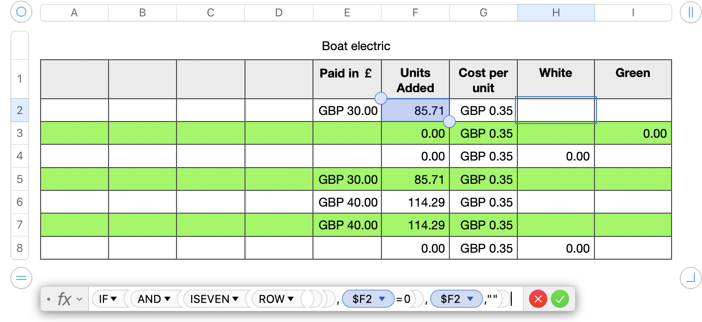
Formula in H2 =IF(AND(ISEVEN(ROW()),$F2=0),$F2,"")

If the row number is even, and the value in F=0, then insert the value from column F. Else insert "" (NULL).

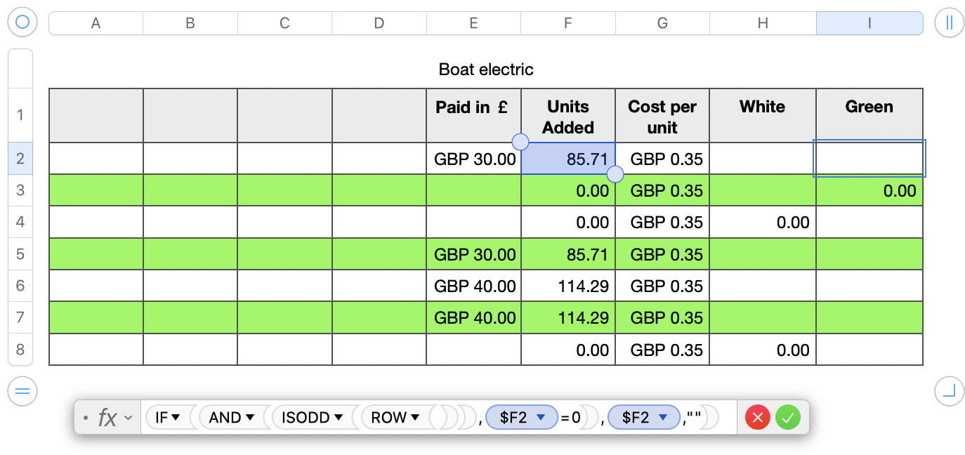
Formula in I2 =IF(AND(ISODD(ROW()),$F2=0),$F2,"")

If the row number is odd, and the value in F=0, then insert the value from column F. Else insert "" (NULL).

Now for the Conditional Highlighting. Select all the body cells in column F. Two rules.

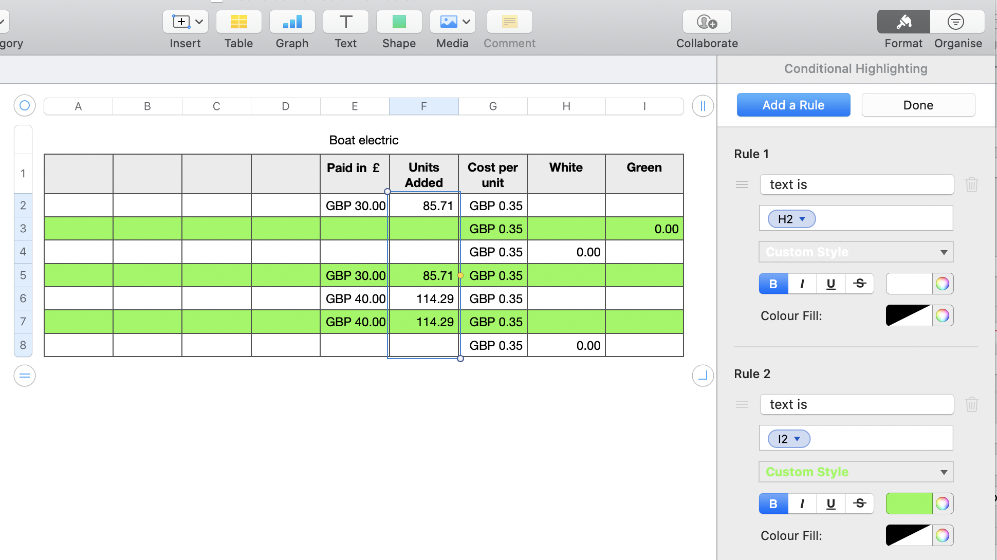
If the text in F is the same as the text in H, then make the text in F white (to match the cell background).

If the text in F is the same as the text in I, then make the text in F green (to match the cell background).

I used Colour Window > Crayons > Lime. Adjust to match your table.

Regards,

Ian.