You can make a difference in the Apple Support Community!

When you sign up with your Apple Account, you can provide valuable feedback to other community members by upvoting helpful replies and User Tips.

Looks like no one’s replied in a while. To start the conversation again, simply ask a new question.

Help with numbers!

I am looking for some help.


I have made up a couple sheets to look like the sheets that I will be using. I am trying to figure out how I can get the information from the first sheet to fill in on the second sheet.


I want the second sheet to fill in with the percentage that that student scored on a particular item. I feel like there has to be a way I just don't know what it is. I also could be totally wrong.


I have no control over the setup of the first sheet with the percentages listed but can control the setup of the other sheet. I just don't know how to go about this. I have tried lookup, Vlookup, Hlookup, index and match. I can't make any of it work.


Posted on Jun 1, 2020 2:48 PM

Reply
Question marked as Top-ranking reply

Posted on Jun 1, 2020 7:04 PM

Hi Eric,


The complication of retrieving the data is that there are two parts—student name and class number—associated with each value in column labelled "Your Percentile"*


You note that you have no control over the setup of the data table.

Can you make alterations to that table after receiving it?


If so, I would suggest adding one column to that table, labelling it 'search', entering this formula in row 2, and filling it down to the end of the added column.

To use VLOOKUP, the added column would need to be inserted to the left of column D (Your Percentile*)

To use MATCH and INDEX the new column could be placed anywhere in the table, including to the right of the last existing column.

Placed in a new column between C (Course Name) and D, the column would become the new column D, and all columns to the right would be bumped up one letter in the alphabet.

Here's a pair of examples using a compacted version of your data table and two summary tables, one using VLOOKUP, the other MATCH and INDEX. The error triangles are all 'can't find' errors due to that student/class combination not being listed in Data.
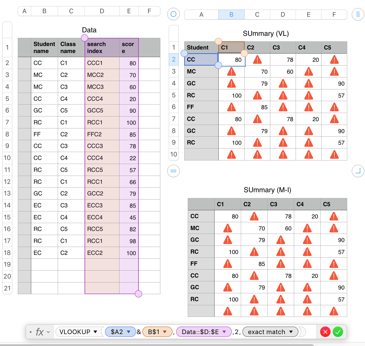
There is one formula on Data, entered in D2 (an added column) and filled down to the end of column D.


D2: B2&C2


The formula is a simple concatenation, which joins the text in column B and the text in column C (with no space between them) into a single string to use as the search for value in VLOOKUP or MATCH. (I've shortened the names to avoid excessive typing and inevitable typing errors, These names (student and class) must exactly match the labels in column A and row 1 of the summary tables.)


Summary (VL) has one formula, shown below the tables. It is entered in B2, filled down to the end of column B, and filled right to column F.


B2: VLOOKUP($A2&B$1,Data::$D:$E,2,FALSE)


SUMMARY (M-I) uses a different formula, entered and filled as described above.


B2: INDEX(Data::$E,MATCH($A2&B$1,Data::$D,0))


Both return the same results.


The error triangles can be avoided by wrapping whichever of the formulas you choose to use in an IFERROR statement:


B2: IFERROR(formula,"")


Place whatever text you want to see for missing student/class combination between the quotation marks. With nothing between them, the formula returns a null string, and the cell appears empty.


I would caution against including IFERROR before you have the formula returning expected results. Error traps like this catch ALL errors, not just the expected ones.


If you are not able to add a column to the Data table after receiving it, create a two column Auxiliary table to construct and contain the search-for values and the score values, then revise the VLOOKUP or MATCH-INDEX formula to use that table.
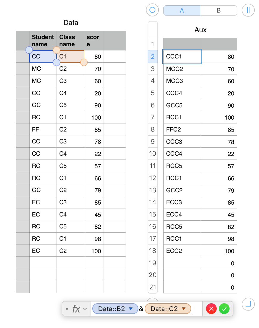
The formula below the table is entered in A2.

B2 contains a simple formula—a cell reference to D2 on the original Data table (no added column).

Both are and filled down as many rows as there are data on the Data table.


Regards,

Barry


5 replies
Question marked as Top-ranking reply

Jun 1, 2020 7:04 PM in response to ericfromwestmoreland

Hi Eric,


The complication of retrieving the data is that there are two parts—student name and class number—associated with each value in column labelled "Your Percentile"*


You note that you have no control over the setup of the data table.

Can you make alterations to that table after receiving it?


If so, I would suggest adding one column to that table, labelling it 'search', entering this formula in row 2, and filling it down to the end of the added column.

To use VLOOKUP, the added column would need to be inserted to the left of column D (Your Percentile*)

To use MATCH and INDEX the new column could be placed anywhere in the table, including to the right of the last existing column.

Placed in a new column between C (Course Name) and D, the column would become the new column D, and all columns to the right would be bumped up one letter in the alphabet.

Here's a pair of examples using a compacted version of your data table and two summary tables, one using VLOOKUP, the other MATCH and INDEX. The error triangles are all 'can't find' errors due to that student/class combination not being listed in Data.

There is one formula on Data, entered in D2 (an added column) and filled down to the end of column D.


D2: B2&C2


The formula is a simple concatenation, which joins the text in column B and the text in column C (with no space between them) into a single string to use as the search for value in VLOOKUP or MATCH. (I've shortened the names to avoid excessive typing and inevitable typing errors, These names (student and class) must exactly match the labels in column A and row 1 of the summary tables.)


Summary (VL) has one formula, shown below the tables. It is entered in B2, filled down to the end of column B, and filled right to column F.


B2: VLOOKUP($A2&B$1,Data::$D:$E,2,FALSE)


SUMMARY (M-I) uses a different formula, entered and filled as described above.


B2: INDEX(Data::$E,MATCH($A2&B$1,Data::$D,0))


Both return the same results.


The error triangles can be avoided by wrapping whichever of the formulas you choose to use in an IFERROR statement:


B2: IFERROR(formula,"")


Place whatever text you want to see for missing student/class combination between the quotation marks. With nothing between them, the formula returns a null string, and the cell appears empty.


I would caution against including IFERROR before you have the formula returning expected results. Error traps like this catch ALL errors, not just the expected ones.


If you are not able to add a column to the Data table after receiving it, create a two column Auxiliary table to construct and contain the search-for values and the score values, then revise the VLOOKUP or MATCH-INDEX formula to use that table.

The formula below the table is entered in A2.

B2 contains a simple formula—a cell reference to D2 on the original Data table (no added column).

Both are and filled down as many rows as there are data on the Data table.


Regards,

Barry


Jun 1, 2020 8:10 PM in response to Barry

Barry,


Thank you so much, this has been making me NUTS! Works can not express how thankful I am!


I just have one additional question if I am not pushing my luck... what does the ,2, mean in the formula? I was thinking it means the second column in the range? But it only works with ,2, it doesn't work by selecting the entire column. I got confused. I could be tired too.


Jun 3, 2020 6:13 AM in response to ericfromwestmoreland

I'd skip the intermediate tables and just use one formula in B2, filled right and down:


=SUMIFS(Table 1::$D,Table 1::$B,$A2,Table 1::$C,B$1)


You'd get the same result using:


=AVERAGEIFS(Table 1::$D,Table 1::$B,$A2,Table 1::$C,B$1)


This works assuming there is only one score for each User Course pair (i.e., I assume in your example Ritz Cracker/Class 1 and Cheddar/Class 4 were duplicated in error) because taking a sum or average of one value equals that value.


SG


Jun 1, 2020 7:38 PM in response to Barry

A math note:


the data table you receive labels coumn D as Y0ur Percentile, but formats the data as Percentages. They're not the same.


Suppose 100 students wrote the same 100 question test.

99 of the students answered 25 questions correctly. Their percentage was 25%. Their scores were at the 99th percentile.

The other student answered 24 questions correctly. His percentage was 24%. His score was at the 1st percentile.


Now suppose the low scoring student asked to have his test reviewed, and on review two more questions had been answered correctly by that student.


His percentage is now 26%. And his score is now it the 100th percentile.

The 99 other students' percentage was still 25%. There score was now at the 99th percentile.


Regards,

Barry


Jun 1, 2020 10:47 PM in response to ericfromwestmoreland

Hi Eric,


Your thoughts on 2 are correct.


The lookup table, in this case is columns D and E of Data .


The original LOOKUP function had you specify a column in which to search and a column from which to return the value in the same position as it found the search value in the search column.


VLOOKUP has a different syntax: You define the range of columns that make up the lookup table (Data::D:E ) at the start. VLOOKUP always searches in the leftmost column of that table (Data::D ) then returns the same row value from the column you define by number, where 1 is the search column, 2 is the column to the right of the search column, etc. up to the last column specified as being in the lookup table.


You can find the syntax of every function supported in Numbers in the Function Browser. You'll also fnd a description of the funcion, and at least one example of how it can be used in a Numbers document.


To open the browser, select any cell in a Numbers table, then type =


This opens the Formula editor at the cell AND the Function Browser in the right sidebar.

Typing vl in the browser's Search box will bring up the article on VLOOKUP.


One other note regarding formulas and notation: The "cell references: Use Header names as labels" works well when the formula is being read by it's author, but slows things down when someone unfamiliar with your table is analyzing a formula.

Most of the people expressing a preference here have asked that the feature be turned off for screenshots to provide a quicker view of the structure of the formula and the table.


Regards,

Barry

Help with numbers!

Welcome to Apple Support Community
A forum where Apple customers help each other with their products. Get started with your Apple Account.