Weighted Average Date

Dates in MS Excel are stored as serial numbers counting the days since a specific 'day 1'.

Dates in Numbers are the date part of a Date and Time string marking a specific point in the flow of time.

Setting a 'start date' then counting days from that date to each of the deposit dates gives us a list on numbers which can be used with the deposit amount to calculate a SUMPRODUCT value that can be used to determine the weighted average date using a formula much like the provided Excel example.

Row 1 is a Header Row.

Row 10 is a Footer Row.

(Column A is a Header column, but this is not significant for this table.)

Columns A and C, rows 1 to 9 are copied from your example.

Column B contains a 'starting date' in B1, and the formula below, entered in B2 and filled down to B9. The formula converts the date part of the Date and Time value in its row of column A to a number showing the number of days from the date in B1 to the date in 'this row' of column A.

B2: DATEDIF(B$1,A2,"D")

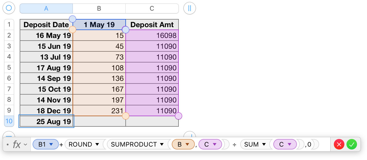
The weighted average date is calculated by the formula shown below the table in the image above. The formula is in cell A10 of the table.

A10: B1+ROUND(SUMPRODUCT(B,C) ÷ SUM(C),0)

Defining row 1 and a Header row and row 10 as a Footer row allows using the letter only references for columns B and C in the formula.

Both SUM and SUMPRODUCT read these references to mean 'all cells in the column, excluding cells in header or footer rows.'

Regards,

Barry

Yes, Numbers stores dates as a date-time strings (which can't be used in SUMPRODUCT) whereas Excel stores them as integers. The Numbers approach is convenient in many situations but a little less convenient than Excel in this situation.

One way to approach this in Numbers would be to add a column (which can later be hidden) and do something like this:

The formula in B2 of Table 1, filled down:

=A2−DATE(YEAR(A2)−1,12,31)

The formula in B2 of Table 1-1:

=DATE(YEAR(Table 1::A2)−1,12,31)+SUMPRODUCT(Table 1::B,Table 1::C)÷SUM(Table 1::C)

This assumes you are looking for a weighted average date within one year, perhaps for estimating investment performance in that year.

If you want a weighted average over a period longer than a year then this formula can be modified. Just post if you need that.

Note that in Numbers, unlike in Excel, it's easy to avoid referencing partial columns. If you put your formula in a separate table (or in a Footer Row in the original table) then you can just reference B rather than having to reference B2:B9, etc.

SG

Just a heads up. I tested my solution above and compared its results to Excel, as shown here:

So if you want the same result as in Excel then you can try my suggested solution above as is, or modify Barry's.😀

SG