Help sought with SUMPRODUCT from an Excel Sheet and displaying only rows containing data?

You can select the rows you don't want to see, right click, and hide them. After printing, unhide them. It isn't automatic but it will hide them without having to delete rows.

Alternatively, rework the sheet so it does not have vertically merged cells. Filters will then be usable.

More rambling followed by how I would replicate the formula in Numbers. It appears I decoded it correctly.

One problem with trying to replicate the formula in Numbers is IEEE 754 binary math. If there are three of a number, each gets assigned the number 1/3. The number 1/3 cannot be created exactly, it is represented as 0.3333333333333330. Add three of them together in Numbers and you don't get exactly 1, you get 0.9999999999999990. You have to display a lot of decimals to see this. This will throw off the rest of the math. In Excel, that little error is corrected and you do get 1 exactly. However, in Excel if you actually have the numbers 0.3333333333333330 and added three of them, the result might be 1 or 0.9999999999999990 depending on how you created those numbers. You have to be aware of these things when dealing with decimal numbers and fractions. They can mess things up. Excel and Numbers don't always do the same thing.

ROUND can fix that little math error in Numbers but I don't like relying on it. Or maybe there are only 1 or 2 of a number so the problem with 1/3 never comes up. The replicated formula, which actually requires a column of formulas, would be:

B14 =IF(A14<>"",1/COUNTIF(A$14:A$47,A14),"")

fill down to B47

The formula for summing these results and doing the rest of the math =INT((ROUND(SUM(B14:B47),0)+1)/2)

A better set of formulas that does not have any math issues, and is simpler too, would be

B14 =COUNTIF(A$14:A14,A14)=1

fill down to B47

The formula for summing these results and doing the rest of the math =INT((COUNTIF(B14:B47, TRUE)+1)/2)

Hide column B after it is all set up.

If you add more rows, the formula in column B will automatically fill to the new rows. If you always add those new rows by inserting rows above row 47, the summation formula will adjust to include the new rows.

You don't have to use column B for the column of formulas, you can do this in a column far off to the right if you want to.

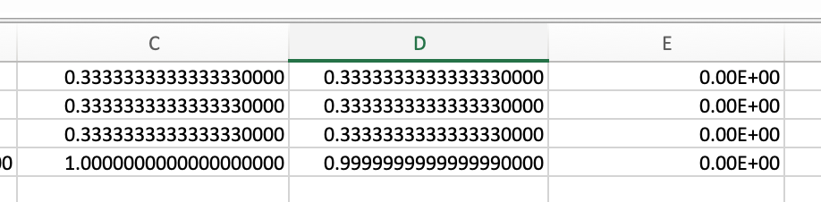
Back to rambling, below is Excel giving two different results for the same numbers. The 0.333's in column C were pasted formula results from a cell that had 1/3 in it. Column D I typed in the numbers. Column E = C-D and it equals 0 exactly, indicating that C and D have the exact same numbers in them. But the sums at the bottom of C and D are obviously different.

There is almost certainly a way to approach this in Numbers, but it difficult to reconcile the formula in your post with the description of what it does (number from 1-99, etc). Perhaps you could post an example, giving some context about what you are trying to do.

SG

what rows in a sheet are occupied by a number from 1-99 and where they are, count those then perform a second sum of dividing the total by 2 and rounding up.

INT((SUMPRODUCT((A14:A47≠"")÷COUNTIF(A14:A47,A14:A47&""))+1)÷2)

I have to think out loud to put this together. You don't have to read it, just skip to the end with what I think this formula's results actually are.

(A14:A47≠"") is the same as having a column of formulas next to A14-A47 starting with =IF(A14<>"",TRUE,FALSE). It creates an internal array vs having a column in the table. It is an array indicating whether that row had a value in it or not. TRUE will be treated as a 1 and FALSE as 0 in the math formula coming up.

COUNTIF(A14:A47,A14:A47&"") is, I believe, the same as having a column of formulas next to A14-A47 starting with =COUNTIF(A$14:A$47,A14&"") which counts how many of that particular value are found in A14-A47. So if A14-A47 had five values equal to "2", those five rows would get a "5" from this formula.

Dividing the first by the second is like dividing "is there a value in this row (1 if there is, 0 if not)" by "how many of this value are in A14-A47".

The SUMPRODUCT is not really doing a "sumproduct", it is just doing a simple sum of all those answers. I think SUMPRODUCT might be necessary for Excel to do this "array formula" type of formula.

INT rounds down, not up.

So if there were five values equal to 2, each of them would have TRUE in the first array and "5" in the second. The result of the division for each row would be 1/5 and the sum of those results would be 1. The formula then adds another "1" to it and divides by 2 for a final result of 1. If there had been two different values in A14-A47 it would have summed to 2 then + 1 = 3 then divided by 2 = 1.5 and INT = 1.

From what I can tell, then, if there is one unique value in A14-A47 the result should be 1, if two unique values then 1, if 3 unique values then 2, if 4 unique values then 2, etc.. It is not looking for any particular values, there is nothing about 1-99 in the formula, it could be anything in those cells.

I should add that if the formula is doing what I think it is doing, I think it will require at least one column in Numbers. However, if it is doing what you said in the text of your post, that operation could probably be done in one cell.

If there are no missing numbers in the list (for example you will never have 1,1,3,4,etc with no 2), a simple single-cell formula should do the trick. With the all the entries in A14:A47 entered, the numbers can be in any order whatsoever as long as no number is skipped over (missing). The answer may get wonky as data is being entered if the entries are not made in numerical order, though.

=INT((MAX(A14:A47)−MIN(A14:A47)+2)÷2)

If the list always starts with 1, it can be even more simple

=INT((MAX(A14:A47)+1)÷2)