Vlookup help

In another column, you can use the formula

=IF(COUNTIF(B,A)>0, "Value Also Found in Column B", "")

This will flag the rows where the value in column A is also found somewhere in column B. It won't say where it is found, only that it was. A different formula can be used to do the same thing and also point you to the row in column B but if there is more than one occurrence it will only tell you about one of them.

You're welcome, Chris.

One other note on finding the repeated values:

You could do this using conditional highlighting:

Add a tiny table (one header cell and one body cell).

Select columns A and B of the data table, then command click on the header cessa, A1 and B1 to remove them from the selection.

Open the Format Inspector, click Cell, then click Conditional Highlighting (bottom row of the inspector pane).

With all but the first row of columns A and B of the data table still selected, set the rule shown:

Click:

• Add a rule
• Text
• is
• the icon at the right end of the entry box
• cell A2 of the Highlights table

Then click the small triangle in the A2 icon and click to check Protect row and Protect column.

Click the triangle in the box showing bold, and choose a fill colour for the highlighted cells.

Click Done.

Applying the highlights:

In the Highlights table:

• Click cell A2 and enter one of the item numbers that has a count of more than 1 0.
• Click outside that table to confirm the entry

In the main table:

• All cells in columns A and B containing the entered value will now have the highlight colour as their background fill.
• Edit the cells as needed (remembering to not delete the one you want to keep).

Repeat these four steps with each duplicated item number.

Still tedious, but the highlighting will make it easier to spot the cells needing attention.

Regards,

Barry

PS: In answer to your question to BU—All of the above, and most of it hands on.

B.

VLOOKUP,

Like all of the lookup functions, returna a single value from the same row as that in which it finds the search value provided for it.

in VLOOKUP, the search may be set to require an exact match or to accept a close match (largest value less than or equal to the search value).

In LOOKUP, 'close match' is the default and only choice.

In MATCH, the formula can be set to look for 'the value' (exact match), 'largest (same as 'close match') or 'smallest (similar to 'close match', but from the other direction—accepting the smallest value greater than or equal to the search value)

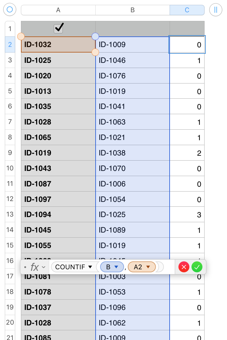
Better for what you want would be the COUNTIF function.

Insert a new column after column B. The new column will become column C.

To count the number of times each value in column A appears in column B, enter this formula in C2:

COUNTIF(B,A2)

The formula is entered as shown in cell C2, then filled down to the end of that column,

The formula answers the question "how many times does the value in A2 appear in column B?

If you include a second COUNTIF, and a couple of spaces between the two copies of the function, you can get a count of that value in each of the two columns:

The first digit in column C shows the number of times the value on 'this row' of column A is found in column A (including the one on 'this row'). The second shows the number of tines the value on this row of column A appears in column B.

The 1  0 in row 7 shows that ID-1096 appears only once in the table.

As before, the formula is entered as shown in C2, then filled down to the end of the table

Missing is a count of how many times each value in column B appears in column A and in column B. This could b added to the formula above, but would probably be more easily read and understood if it were in a separate column. The formula is the same as the one in the table above, with B2 replacing each of the A2 values.

Enter in D2, and fill down.

The values in the example table are generated randomly within a range of only 101 possible values to ensure there will be some repeated values to count. The checkbox in cell A1 of the table is there only to trigger the random ID- formula to re-calculate the numbers, and is not required in your table.

Regards,

Barry

The function to be used is easy to find. The proper way to use it for your problem will not be found there. So here is it:

This one will find the row that has the matching value. If there is more than one matching value, it gives you the one closest to the top of the table.

=IFERROR("Value found in row "&MATCH(A,B,0), "")

A secondary formula that can tell you if there is more than one match is below. It assumes the above formula is in column C

IF(C<>"", IF(XMATCH(A,B,0,1)<>XMATCH(A,B,0,−1),"More than One Match", ""), "")

Yeah duh COUNTIF .I got my head stuck in MATCH.