You can make a difference in the Apple Support Community!

When you sign up with your Apple Account, you can provide valuable feedback to other community members by upvoting helpful replies and User Tips.

Looks like no one’s replied in a while. To start the conversation again, simply ask a new question.

Numbers Formula Assistance Needed

I have a commission structure that I am attempting to create a formula for.

The Tier levels are as follows

$0 - $20,000 sold is 10% commission of sale price

$20,000.01 - $30,000 sold is 15% commission of sale price

$30,000.01 - $40,000 sold is 20% commission of sale price

pattern continues.


I had this set up with this formula in each tier level column

ex: E12 was VLOOKUP(SUM(D$5:D12),$H$6:$I$64,2,1)

ex: E13 was VLOOKUP(SUM(D$5:D13),$H$6:$I$64,2,1)


The problem is this:

if I am at $18,000 in sales, and I sell a $3000 product, then $2000 of that would be 10% and $1000 would be 15%.

I am not sure how to do that with the formula.

MacBook Pro 15″, macOS 10.15

Posted on Dec 15, 2020 7:50 AM

Reply
Question marked as Top-ranking reply

Posted on Dec 16, 2020 4:14 PM

HI auldenzuck,


Here's an example that should work for you.


The tier level is based on the total sales, so calculations need to be based on that as well, meaning we need a column in which each row has a cell showing total sales after the current sales recorded in column C, and a column on the Rates table showing the (total) amount of commission that has (or will have been) paid when each threshold value has been reached.
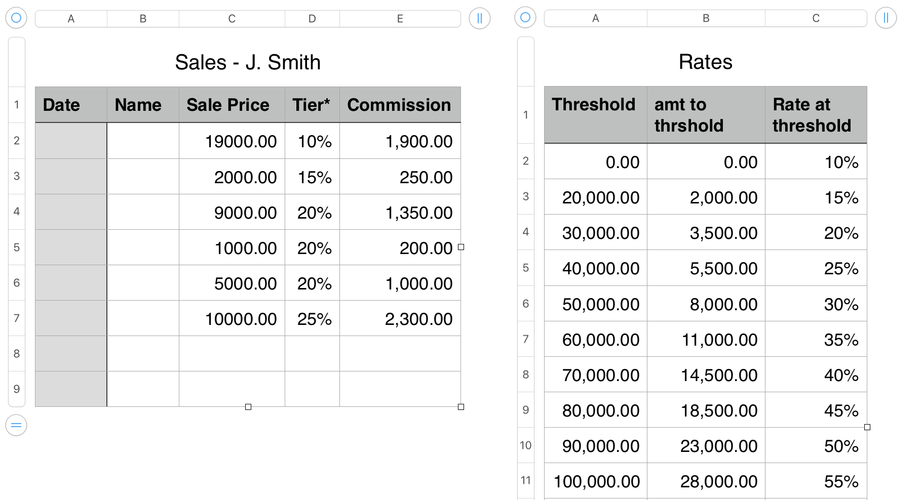

Above is a general image of the two tables as they would appear is use. The Rates table can be placed on a sheet separate from the one holding the Sales table. If there are more than one sales person, and the commission schedule is the same for each, all of the Sales tables (each with a name that includes the name or other ID for the person) can reference the same Rates table.


The Rates table contains entered data in columns A and C, and in row 2 of column B. The formula shown in the image below is entered in B3, and filled down to the end of column B.
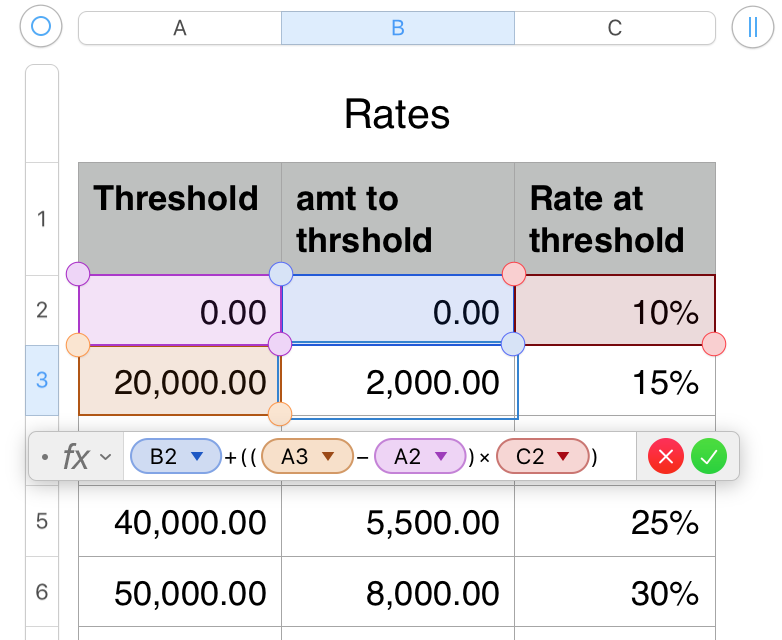

B3:   B2+((A3−A2)×C2)


The formula gets the amount of commission paid up to the threshold value in the row above, then multiplies the difference between the threshold value on 'this row' and on the row above by the commission rate of that tier.


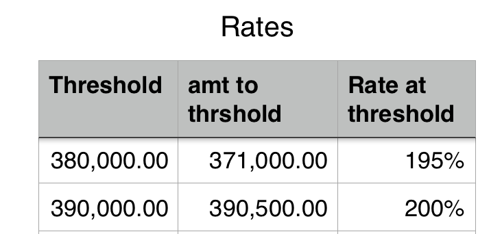
A note of interest: If the "pattern continues" indefinitely, total commissions will exceed total sales when cales reach this level:
The Sales table has two hidden columns that calculate the total sales and total commissions to each row, figures necessary for the calculations on this table.
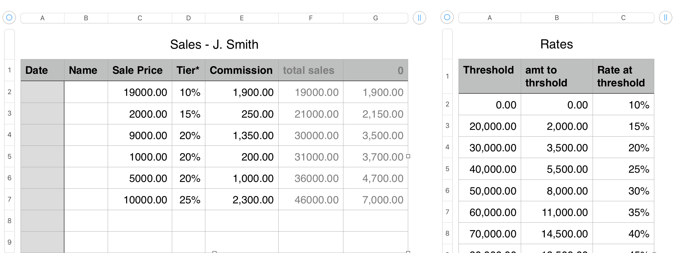

Columns A and B and C contain entered data. A and B are left empty as they do not enter into the calculations in the other cells.

Column D contains a lookup formula that uses the Total sales amount in in column E to determine which is the largest threshold value in column A of Rates that has been reached, and returns the commission rate from column C of the same row of Rates.


The Vlookup formula is wrapped in an IF statement that precents the calculation until there is an entry on 'this row' of column C, and places a null string in the cell, making it appear 'blank' (rows 8 and 9). This same wrapper is applied to the formulas in columns E, F and G of this table.
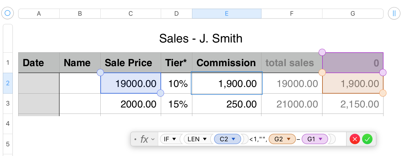

Column F contains one of the simplest formulsa on the table. It calculates the commission on the current sale by subtracting the commissions paid up to the previous row (G1 in the example) from those due on the total sales to 'this row' (in G2).

The 0 in G1 is an entered value. those in G2 , G3 and on down are calculated.
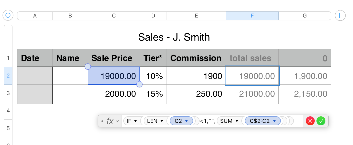

The other 'simplest' formula on the table is this one, plsced in column F. SUM uses an 'expanding range' to get the values in column C from C2 (fixed) to 'this row' of column C, and returns the sum of those values.


Which brings us to column G, where the total commissions to 'this row' are calculated and stored.
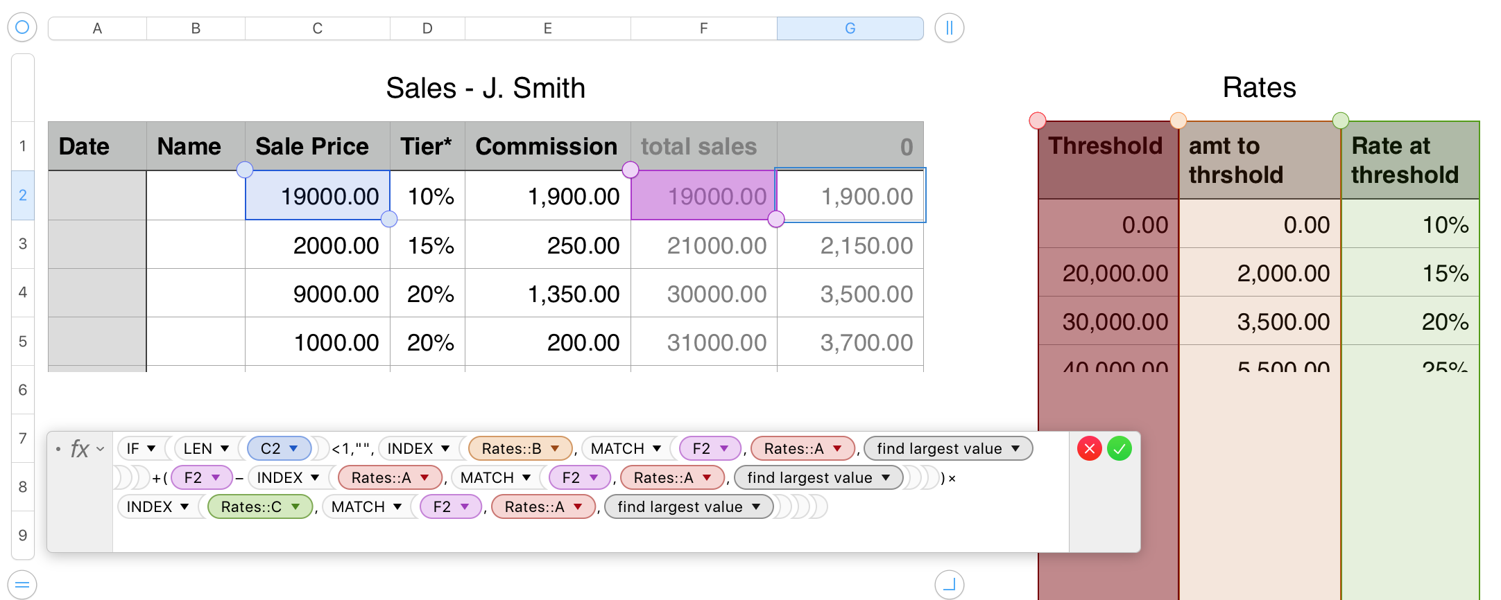


Skipping the IF switch common to all of the formulas on this table, the formula uses three INDEX— MATCH pairs to gather three values


,INDEX(Rates::B,MATCH(F2,Rates::A,1))

gets the amount of commission paid and due up to the current threshold total sales value


+(F2−INDEX(Rates::A,MATCH(F2,Rates::A,1)))

gets the current total sales value from column F and subtracts the current threshold value to determine the amount subject to this tier's commission rate.


×INDEX(Rates::C,MATCH(F2,Rates::A,1))

gets the commission rate for this tier from column C of Rates and multiplies the second result by this rate to get the commission due in this tier.


The result of the multiplication is added to the amount due at the last threshold.


The sum is the current Total Commission (due or paid) for total sales including this transaction.


Copy//paste versions of the formulas:


Rates:


B3: B2+((A3−A2)×C2)


Sales:


D2: IF(LEN(C2)<1,"",VLOOKUP(F2,Rates::A:C,3,close-match))


E2: IF(LEN(C2)<1,"",G2−G1)


F2: IF(LEN(C2)<1,"",SUM(C$2:C2))


G2: IF(LEN(C2)<1,"",INDEX(Rates::B,MATCH(F2,Rates::A,1))+(F2−INDEX(Rates::A,MATCH(F2,Rates::A,1)))×INDEX(Rates::C,MATCH(F2,Rates::A,1)))


Regards,

Barry


Note: INDEX—MATCH formulas could be replaced with VLOOKUP versions performing the same task. See the Sales, column D formula for a model.

B.


6 replies
Question marked as Top-ranking reply

Dec 16, 2020 4:14 PM in response to aldenzuck

HI auldenzuck,


Here's an example that should work for you.


The tier level is based on the total sales, so calculations need to be based on that as well, meaning we need a column in which each row has a cell showing total sales after the current sales recorded in column C, and a column on the Rates table showing the (total) amount of commission that has (or will have been) paid when each threshold value has been reached.


Above is a general image of the two tables as they would appear is use. The Rates table can be placed on a sheet separate from the one holding the Sales table. If there are more than one sales person, and the commission schedule is the same for each, all of the Sales tables (each with a name that includes the name or other ID for the person) can reference the same Rates table.


The Rates table contains entered data in columns A and C, and in row 2 of column B. The formula shown in the image below is entered in B3, and filled down to the end of column B.


B3:   B2+((A3−A2)×C2)


The formula gets the amount of commission paid up to the threshold value in the row above, then multiplies the difference between the threshold value on 'this row' and on the row above by the commission rate of that tier.


A note of interest: If the "pattern continues" indefinitely, total commissions will exceed total sales when cales reach this level:

The Sales table has two hidden columns that calculate the total sales and total commissions to each row, figures necessary for the calculations on this table.


Columns A and B and C contain entered data. A and B are left empty as they do not enter into the calculations in the other cells.

Column D contains a lookup formula that uses the Total sales amount in in column E to determine which is the largest threshold value in column A of Rates that has been reached, and returns the commission rate from column C of the same row of Rates.


The Vlookup formula is wrapped in an IF statement that precents the calculation until there is an entry on 'this row' of column C, and places a null string in the cell, making it appear 'blank' (rows 8 and 9). This same wrapper is applied to the formulas in columns E, F and G of this table.


Column F contains one of the simplest formulsa on the table. It calculates the commission on the current sale by subtracting the commissions paid up to the previous row (G1 in the example) from those due on the total sales to 'this row' (in G2).

The 0 in G1 is an entered value. those in G2 , G3 and on down are calculated.


The other 'simplest' formula on the table is this one, plsced in column F. SUM uses an 'expanding range' to get the values in column C from C2 (fixed) to 'this row' of column C, and returns the sum of those values.


Which brings us to column G, where the total commissions to 'this row' are calculated and stored.


Skipping the IF switch common to all of the formulas on this table, the formula uses three INDEX— MATCH pairs to gather three values


,INDEX(Rates::B,MATCH(F2,Rates::A,1))

gets the amount of commission paid and due up to the current threshold total sales value


+(F2−INDEX(Rates::A,MATCH(F2,Rates::A,1)))

gets the current total sales value from column F and subtracts the current threshold value to determine the amount subject to this tier's commission rate.


×INDEX(Rates::C,MATCH(F2,Rates::A,1))

gets the commission rate for this tier from column C of Rates and multiplies the second result by this rate to get the commission due in this tier.


The result of the multiplication is added to the amount due at the last threshold.


The sum is the current Total Commission (due or paid) for total sales including this transaction.


Copy//paste versions of the formulas:


Rates:


B3: B2+((A3−A2)×C2)


Sales:


D2: IF(LEN(C2)<1,"",VLOOKUP(F2,Rates::A:C,3,close-match))


E2: IF(LEN(C2)<1,"",G2−G1)


F2: IF(LEN(C2)<1,"",SUM(C$2:C2))


G2: IF(LEN(C2)<1,"",INDEX(Rates::B,MATCH(F2,Rates::A,1))+(F2−INDEX(Rates::A,MATCH(F2,Rates::A,1)))×INDEX(Rates::C,MATCH(F2,Rates::A,1)))


Regards,

Barry


Note: INDEX—MATCH formulas could be replaced with VLOOKUP versions performing the same task. See the Sales, column D formula for a model.

B.


Dec 16, 2020 5:11 PM in response to aldenzuck

If you have a limited number of tiers, you can also do it the way shown below. The biggest downside is the commission schedule is hard coded into the formulas vs in a table where it can be more easily changed. The second downside is it is only useful for a tiered system that has a small number of tiers, not one where "the pattern continues".


I do wonder about a commission schedule that is so large. If the pattern continues, it could be more than 100% of the sale. Whether someone could actually achieve that tier or not doesn't really matter, it is not good practice to present it. Someone will find a way to get there, by hook or by crook.


Assuming we cap the commission schedule at 30% for >=$50,000K

F2 =IF(D2<>0,H2−H1,"")

G2 =SUM(D$2:D2)

H2 =G2×10%+MAX(0,G2−20000)×5%+MAX(0,G2−30000)×5%+MAX(0,G2−40000)×5%+MAX(0,G2−50000)×5%

Fill down to complete the columns.

Hide columns G and H


Column H is total commission earned so far. There is no text in the header cell because we need that cell to =0. The percentages in the formula are the increases from the previous tier to the next, which happens to be 5% each time.


For the "tier" column, it didn't seem right to display the top tier they hit so it is showing the effective tier for this particular commission.

E2 =F2/D2

or, to avoid divide by zero errors

=IF(D2<>0,F2/D2,"")

Fill down to complete the column


If what you want is the top tier achieved, the formula would be

=IFS(G2≥50000,30%,G2≥40000,25%,G2≥30000,20%,G2≥20000,15%,TRUE,10%)

This does, of course, hard code the tier schedule in a second formula, doubling your chances of messing up if you later want to change it.


Numbers Formula Assistance Needed

Welcome to Apple Support Community
A forum where Apple customers help each other with their products. Get started with your Apple Account.