Formula for multiple IF conditions

Question

Level 1

8 points

Formula for multiple IF conditions

Hi, guys,

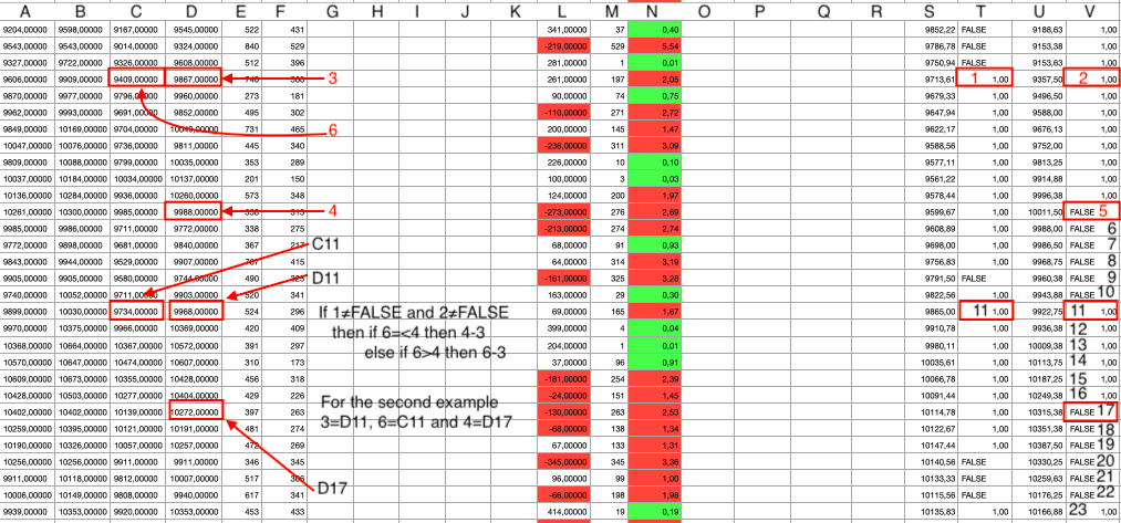
I need you help. I have the following situation: nothing happens when the columns which contain the (1) and (2) cells are FALSE. Then, both columns ≠ FALSE, so, both contain values. Therefore, when the column which contains the cell 2 change its value to FALSE (5) once again, then the below formula takes place. Is there any way in which I can create a formula for this kind of situation?

P.S. I need to mention that there's no fixed number of cells between the moment when both columns are FALSE and when FALSE appears once again in the column which contains the cell 2.

Thank you!

Posted on Jul 19, 2021 6:00 PM

Reply

Answer 1

Top-ranking reply

Badunit

Level 7

28,024 points

Jul 20, 2021 6:47 AM in response to mihai179

One more question to start: are all those 1.00's in columns T and V supposed to be "true" or do you want them to be 1.00?

Here is an attempt at the solution. It is way too difficult to do it in one column. It could be done but the formula would be horrendous. I broke it into multiple columns. You will have to determine if I (and you) got the logic correct. That is a lot easier to do with it broken down into smaller parts in separate columns. You can look at each column and see if the logic/formula for that column is doing what you want it to do.

W2 =AND(V2=FALSE,V1<>FALSE,V2<>"")

This formula flags the rows where V goes from "not false" to FALSE. This will be the "#4 #5" row

X2 =AND(T2<>FALSE,V2<>FALSE,OR(T1=FALSE,V1=FALSE))

This flags the rows where T and V both become "not false". This will be the "#6 #3" row

Y2 =XLOOKUP(TRUE,$X$2:$X2,C$2:C2,"",0,−1)

This formula gets the correct "#6" value

Z2 =XLOOKUP(TRUE,$X$2:$X2,D$2:D2,"",0,−1)

This formula gets the correct "#3" value

AA2 =IF(W2,IF(Y2≤D2,D2−Z2,Y2−Z2),"")

This is IF formula with the end result

Put all those formulas in row 2 then select them all and drag/fill or copy/paste to the bottom of the table.

You can hide columns W-Z later.

Reply

Answer 2

mihai179 Author

Level 1

8 points

Jul 20, 2021 4:24 PM in response to Badunit

Thank you! I still have a small problem with this formula: Y2 =XLOOKUP(TRUE,$X$2:$X2,C$2:C2,"",0,−1) This formula gets the correct "#6" value.

I replaced:

"," with ";"
X with AD (AD is the related column from my file)
C with E (E is the related column from my file)

So, my formula looks like this: Y2 =XLOOKUP(TRUE;$AD$2:$AD2;E$2:E2;"";0;−1) and the first 47 entries are empty and then, it seems that the same value repeat itself for a while and then another value repeat itself for a while and so on. I think I did something wrong when I changed the formula. Am I right? Thank you!

Reply

Answer 3

mihai179 Author

Level 1

8 points

Jul 20, 2021 5:22 AM in response to Badunit

Hi,

Thank you for your prompt answer. I found the email from Apple Support Communities in spam, so please accept my apologies for the delay. Also, accept my apologies for the mess from my message. I added a new image with each column noted. I will answer each question below.

Will all rows have this formula? What column is it to be in? Or is the formula somewhere else and has to determine which row is the one with #6 and #3 as well as which is the row with #4? If the second one, how will it know which is the correct "6 & 3" row?

The formula will stay in a new column near the V column. Let's call it W column.

The formula should be inserted always at the same level with the cell that I noted with 5 in the V column. This is each time the V column become FALSE after a sequence of values or at least one value after both columns (T and V) become TRUE. If I get a FALSE value in V5, then my formula will be placed in W5. So, the formula will start again with T11 and V11 (both are TRUE), and the formula will be inserted in the W17 (because the next FALSE value is located in the V17). This means that 6 & 3 are now like this: 6=C11, 3=D11 and 4=D17. We use now C11 and D11 because T11 and V11 are the starting point for the second formula, and we use D17 because V17 is the next FALSE value from V column.

Therefore, "6 & 3" rows are always at the same level with the first row which has both 1 & 2 rows are TRUE. The 4 is always in the same row with 5.

You said what to do if 1=TRUE and 2=TRUE, you requested "nothing happens" when 1=FALSE and 2=FALSE but what to do if 1=FALSE or 2=FALSE and the other is TRUE?

When 1=FALSE or 2=FALSE and the other is TRUE is the same situation as both are FALSE.

You requested "nothing happens when the columns which contain the (1) and (2) cells are FALSE". A formula cannot do "nothing", it has to give a result in every case. The result can be a null string, so the cell looks blank, that's about as close to "nothing" as can be done. What do you mean by "nothing happens"?

By "nothing happens" I mean that I am only interested in the situation in which both columns are TRUE. In all the other cases, it would be helpful to have only white cells.

It is helpful if the column letters and row numbers are shown in the screenshot. It is difficult if not impossible to give the correct formula without knowing what the columns and rows are. We can give an example formula that you can edit to fit your actual table, but not one that you can simply copy/paste into your table.

I really hope that the second screenshot is more suitable. I noted each column with a letter and I counted the rows on the right side starting with 5.

Thank you again!

Reply

Answer 4

mihai179 Author

Level 1

8 points

Jul 21, 2021 2:30 AM in response to Badunit

Hi and thank you for all your help and patience. I entered everything right but for some reason I get this result: 6≤4⇒6-3 even if in this case 6≤4, the formula looks good and the outcome should be: 6≤4⇒4-3. Any thoughts? Thank you again!

Reply

Answer 5

Badunit

Level 7

28,024 points

Jul 19, 2021 7:02 PM in response to mihai179

Happy to help but there are some questions before an answer can be provided. Depending on the answers it may be a few rounds of questions.

Will all rows have this formula? What column is it to be in? Or is the formula somewhere else and has to determine which row is the one with #6 and #3 as well as which is the row with #4? If the second one, how will it know which is the correct "6 & 3" row?

You said what to do if 1=TRUE and 2=TRUE, you requested "nothing happens" when 1=FALSE and 2=FALSE but what to do if 1=FALSE or 2=FALSE and the other is TRUE?

You requested "nothing happens when the columns which contain the (1) and (2) cells are FALSE". A formula cannot do "nothing", it has to give a result in every case. The result can be a null string so the cell looks blank, that's about as close to "nothing" as can be done. What do you mean by "nothing happens"?

It is helpful if the column letters and row numbers are shown in the screenshot. It is difficult if not impossible to give the correct formula without knowing what the columns and rows are. We can give an example formula that you can edit to fit your actual table but not one that you can simply copy/paste into your table.

Reply

Answer 6

mihai179 Author

Level 1

8 points

Jul 20, 2021 7:52 AM in response to Badunit

Thank you for the answer. That's correct: all those 1.00's in columns T and V, supposed to be "true". I changed them now to true, so, in T and V column is only TRUE and FALSE now. I also added the formulas that you sent, and I get a syntax error. Thank you!

Reply

Answer 7

Badunit

Level 7

28,024 points

Jul 20, 2021 5:53 PM in response to mihai179

It will return nothing until it sees the first TRUE in column AD. Then it will return the value from that row and will continue to return that value until there is another TRUE in column AD, then it will return the value from that row, and so on. It sounds like your formula is working correctly.

Reply

Answer 8

Badunit

Level 7

28,024 points

Jul 21, 2021 5:56 AM in response to mihai179

One thing I am seeing is that your "numbers" in AE and AF are aligning to the left side of the cells. I cannot tell on what side columns E and F are aligning. Text aligns to the left of the cell, unless you change that setting in the format settings. Actual numbers align to the right side of the cell. When comparing strings (text), the comparison is done alphanumerically. 10 is less than 2 when compared that way. I am a little perplexed with your numbers, though, because they look like they should still end up with the correct result. Regardless, let's start with this.

I am guessing you formatted E and F as text. The formulas in AE and AF then become text because their source is the text from E and F. You can probably leave AE and AF alone in the steps below but I included them just to be sure.

Select columns E, F, AE and AF and change the format to Number with the number of decimal places you want. The numbers in the columns should now all be aligned on the right side of the column. You might have to widen E and F to see them. Scan down the columns to be sure all rows changed (a typo that makes a "number" not a number would cause one to not change to a number). Did that fix it?

Reply

Answer 9

mihai179 Author

Level 1

8 points

Jul 21, 2021 12:54 PM in response to Badunit

All the cells were previously set as Automated. I changed the format as you recommended and even if the values from the AE column are still aligned to the left, everything seems to work perfect. Thank you very, very, very much for your help! I really appreciate it, and it was really, really helpful. THANK YOU!

Reply

Answer 10

mihai179 Author

Level 1

8 points

Jul 20, 2021 8:09 AM in response to mihai179

I changed the first formula a bit from W2 =AND(V2=FALSE,V1<>FALSE,V2<>"") into W2=AND(V2=FALSE;V1≠FALSE;V2≠"") and it seems to work.

Reply

Answer 11

Badunit

Level 7

28,024 points

Jul 20, 2021 9:35 AM in response to mihai179

I see now that all those 1.00's are really 1,00's so, yes, you need to use semicolons where I used commas in the formulas. My poor eyesight while looking at your screenshots.

Reply

Formula for multiple IF conditions

Similar questions