You can make a difference in the Apple Support Community!

When you sign up with your Apple Account, you can provide valuable feedback to other community members by upvoting helpful replies and User Tips.

Looks like no one’s replied in a while. To start the conversation again, simply ask a new question.

Making a Spread Sheet for Monthly Payments.

Is there a formula that can be used with multiple "yes", but get over rides by the next one listed? Meaning:

Person "A" paying rent every month at 100 each month, every time they pay, the Monthly Due item changes to the following Month.

January. 100

February. 0

March. 0

April. 0


Month Due:

February.


(I figured out how to make this go to February via formula, but how do I get it to go to March when February is paid for?)


Posted on Jul 25, 2021 12:42 PM

Reply
Question marked as Top-ranking reply

Posted on Jul 25, 2021 10:04 PM

…or three.


Some notes & comments.


Of the formulas shown here, I'd use the one in my first reply, entered into B1. Here's the image again:

The formula shown below the table is entered in the selected cell, B1.

Numbers highlights the cells referenced by the formula using the sam colours as are in the reference tokens as displayed in the formula editor.

The absolute reference operators ( $ ) are not needed, as this formula is not being filled into other cells.


Note that rows 1 and 2 are Header rows. You can set the number of header rows in a Table using the


Looking at the colour highlighting you can see that Numbers is aware that INDEX needs the A reference in the formula to mean 'ALL rows of column A, including those that are header rows,' and automatically sets the formula to include those two rows.

COUNTIF, on the other hand, counts only values in the body cells, and Numbers automatically sets the B reference to include all cells in the column that are not Header rows. (as shown in the colour highlighting of these cells


That's probaly enough to digest for now.


Regards,

Barry

7 replies
Question marked as Top-ranking reply

Jul 25, 2021 10:04 PM in response to Barry

…or three.


Some notes & comments.


Of the formulas shown here, I'd use the one in my first reply, entered into B1. Here's the image again:

The formula shown below the table is entered in the selected cell, B1.

Numbers highlights the cells referenced by the formula using the sam colours as are in the reference tokens as displayed in the formula editor.

The absolute reference operators ( $ ) are not needed, as this formula is not being filled into other cells.


Note that rows 1 and 2 are Header rows. You can set the number of header rows in a Table using the


Looking at the colour highlighting you can see that Numbers is aware that INDEX needs the A reference in the formula to mean 'ALL rows of column A, including those that are header rows,' and automatically sets the formula to include those two rows.

COUNTIF, on the other hand, counts only values in the body cells, and Numbers automatically sets the B reference to include all cells in the column that are not Header rows. (as shown in the colour highlighting of these cells


That's probaly enough to digest for now.


Regards,

Barry

Jul 25, 2021 1:07 PM in response to JSD1999

Here's one way:

The formula shown below the table is entered in cell B3, then filled down the column.


The 3 makes INDEX skip the first two rows and the last row in which a payment has been made.


COUNTIF counts the number of payments that have been made.


The two values are added, and INDEX returns the month name from that row of column A.


Here's the same table after two more payments are made:


As shown, the table will display an error triangle in B1 when the December payment ins made.


The formula assumes there are no months in which a payment will be missied, and does not check that the amount recorded is correct.


Regards,

Barry

Jul 25, 2021 6:27 PM in response to JSD1999

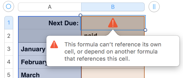
The red error triangle (and the blue 'warning' triangle' always come with a message telling what the error is (or what the warning is about). Click on the triangle to see the message.


In this case, the cause is an error in my post above.


Many (Probably "Most") questions I respond to here use formulas that are calculating values in several cells in a column, and returning the results to each cell in the column.


In this question, the values in B3 and below are all entered directly. The

formula is creating the value to be seen in cell B1, and should be in cell B1, (NOT in B3), and stays in B1 (NOT 'filled down to cells below.)


Specifying the cell range for INDEX as A1:A14 Will work, as will using the same style to specify the cell range to be counted in column B, as can be seen in the example below:


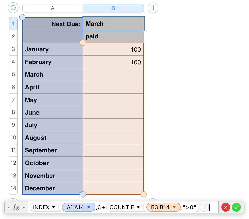
Using this style for defining the range requires that you take care to start the column B range at row 3, something done automatically with the 'letter only' column reference I used in the first example above.


Starting at B1 will produce the error message seen below:


More to come in an hour or two.


Regards,Barry

Jul 25, 2021 2:23 PM in response to JSD1999

Please excuse me as I am new to this program.... I typed in that formula that you provided me in B3 (The box next to January?) and I got an orange error triangle. It may be because when I highlighted all of column A (January-December) It looks like this instead of what your formula looks like: $A1:$A14. Not sure if I am doing that incorrectly as well. Thank you for being patient with me.

Jul 26, 2021 12:05 PM in response to Barry

Barry, I cannot thank you enough for all of the work and time that you put into answering my question, and making me feel so much more comfortable putting this spreadsheet together. I have learned so much, and I’m so excited about it. You are truly amazing, and I appreciate everything! I ended up being successful and pudding the correct formula is in and it works exactly the way I wanted it to! Wishing you nothing but the best; and please stay safe.

Jul 26, 2021 11:02 PM in response to JSD1999

Hi JSD,


You are welcome. And you're welcome to post further quesions when you need further help.


Everyone participating in this community was a 'newbee'' at one time, and know the pains of not knowing. Most of those responding to questions can remember those days, and treat all questions to which they respond as genuine issues that need to be addressed,


Regards,

Barry


Making a Spread Sheet for Monthly Payments.

Welcome to Apple Support Community
A forum where Apple customers help each other with their products. Get started with your Apple Account.