Conditional Highlighting rules in Numbers compare the current value in the cell to be formatted with a fixed value, written into the rule, or to the value in another cell. Since the trigger value is the true or false state of a specific cell, and neither of those values are likely to be in the cell(s) to be highlighted, yu will need to provide a set of cells paired with each of the cells to be highlighted, and manipulate the values in these cells depending on the value in the trigger cell.
Here's an example. "My Tasks" is the table whose rows are to be highlighted when the checkbox cell in column A of that row is checked, indicating the task(s) have been completed.
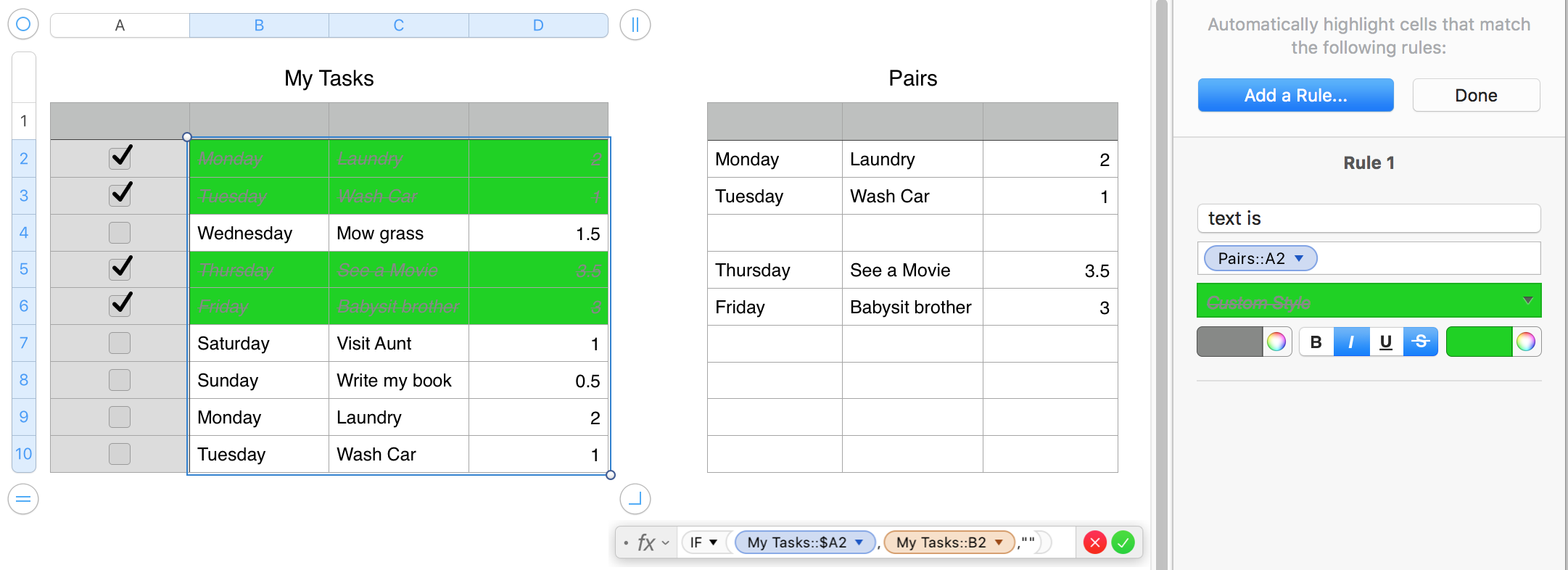
The formula shown below the "Pairs" table is placed in cell A2 to Pairs, and filled down to the bottom of column A, and right to column C.
Checkboxes contain 'true' if they are checked, and 'false' if the box is not checked.
Each copy of the formula gets the value from the checkbox cell in the same row of My Tasks. If that value is 'true' the formula the formula copies the value of its 'paired' cell of My Taske, and pastes it into its own cell. If the checkbox is unchecked, the formula inserts a null string into its cell.
The conditional highlight rule, shown in the right sidebar is set to compare the 'text' displayed in the paired cell for each of the data cells in My Tasks. IF both cells display the same text the rule applies the custom highlighting shown in the rule (strike-through style and a grey colour value is applied to the text, and the cell style is set to green fill in the shade shown.
Where the cell has not been checked, the conditional highlighting is not applied, and the cell and text retain their original style.
Regards,
Barry