muguy has the right function and a correct formula.
These are some additional comments, and a version of the formula that takes advantage of some features of Numbers.
Cells in Numbers with their Data Format set to Checkbox contain one of two boolean values:
true if checked, false if not checked.
The SUM functions (SUM, SUMIF, SUMIFS) and several similar functions omit cells in header rows and footer rows of 'full column' references.
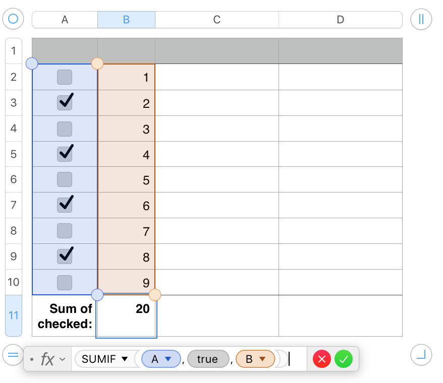
With that in mind, the formula in the example below works well for your purpose:
 The formula shown is in the selected cell, B11. Row 11 is set to be a Footer row, avoiding the self reference error that would occur if this were a normal 'body' row.
When entering the formula, do not enclose true in quotation marks. The Boolean value should appear as shown, even if you type TRUE in the space shown.
A and B are 'full column references for columns A (containing the test values) and B (containing the values to be summed). Note that neither the cells in row 1 (a Header Row) or Row 11 (a Footer row) are highlighted to match the lozenges containing the column references in the formula, indicating the column reference does not include these cells.
If rows are added to or removed from the table, those rows will be placed between the Header row(s) and the Footer row(s), and will be automatically included in (or removed from) the formula.
Regards,
Barry