Name the table on which you are recording the daily sales Data.
Name the second table, on which the monthly totals will be calculated "Summary"
Both tables should have one Header Row, with data entry (and formulas) starting on row 2.
(the table names may be changed AFTER you have entered the formulas below, and have established that they are working correctly. Numbers will automatically revise the formulas to fit the new table names.
Data:
Record the dates in column A.
Record the amounts in column C
Data will contain one formula, entered in column E:
 MONTHNAME(MONTH(A2))&" "&YEAR(A2)
Enter in E2, then fill down to the last cell in the column.
Summary:
Select cells A2:AA13.
Click the Format brush to open the Format Inspector, select Cell, then set the Data format to Text.
Close the inspector.
Enter January in cell A2, then fill down to A13 to add the rest of the month names.
Enter the year number in cell B1
Summary will have two formulas, the first entered in B2, then filled down to to B13:
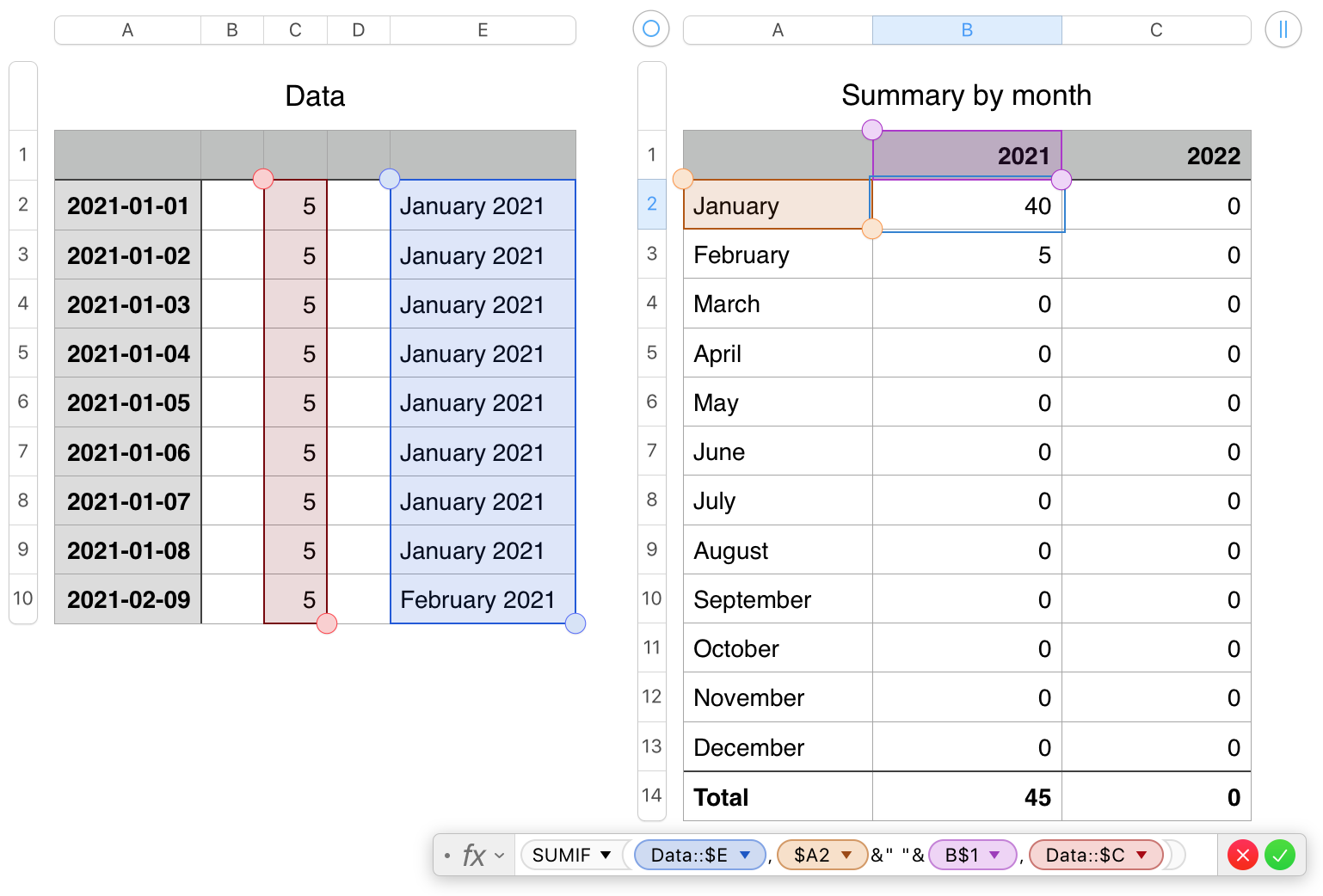
SUMIF(Data::$E,$A2&" "&B$1,Data::$C)
Fill down to row 13, (and right to column C )
Row 14 is added and converted from a 'standard' row to a Footer row. To do the conversion, place the pointer between the Row reference tab of row 14 and the table. Click the v that appears and choose convert to Footer row.
After doing the conversion, click on B14, press = to open the formula editor, and enter SUM(B)
Then click the green checkmark to confirm the formula and close the editor.
With B14 still selected, fill the formula right into column C. (this will probably give you an error message until you place a year number in C1)
IN USE:
Unless you want to see it, Hide Data::E. That information is needed by the SUMIF formula, but not by the user.
You can also hide the 'future' and or 'past' columns on Summary, leaving visible only the current year and any previous years for which you want to do a comparison.
Regards,
Barry