Display cell contents if adjacent cell is true

Here's a method combining a pair of formulas and a filter on the second table.

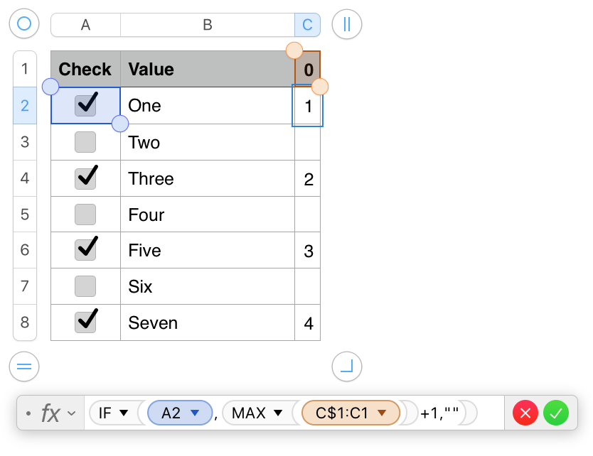
Table 1 has one column added to contain an index of the checkmarked rows, calculated by the formula shown below the table. The new column, C, may be hidden.

The formula is entered in C2, then filled down to the end of that column.

Cell C1 may be empty, or may contain a zero.

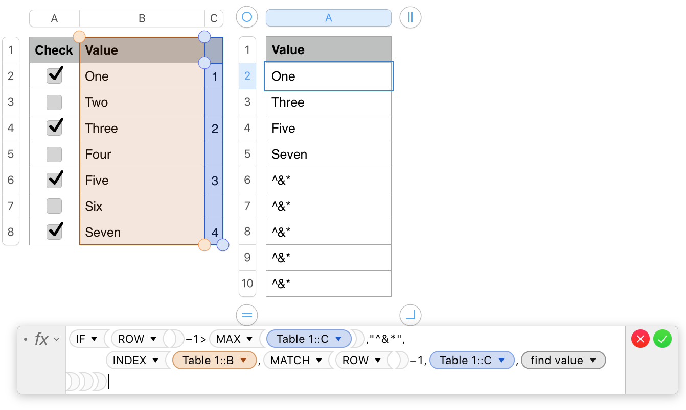
Table 2 may be placed on the same sheet of on a second sheet. Here, for convenience, it is placed beside the first table.

IF(ROW()−1>MAX(Table 1::C),"^&*",
 INDEX(Table 1::B,MATCH(ROW()−1,Table 1::C,0)))

The formula is entered as shown in cell A2 of Table 2, then filled down to the end of the column.

The INDEX/MATCH part (in bold) uses the index numbers in column C of Table 1 to retrieve the values from those rows of column B and place then in consecutive cells here.

The part of the formula in normal weight type is a switch that 'turns off' the bold part when all index values have been found, and places an arbitrary three character text string in the remaining cells of Table 2.

If you're happy with 'empty' cells showing, replace the "^&*" in the formula with "".

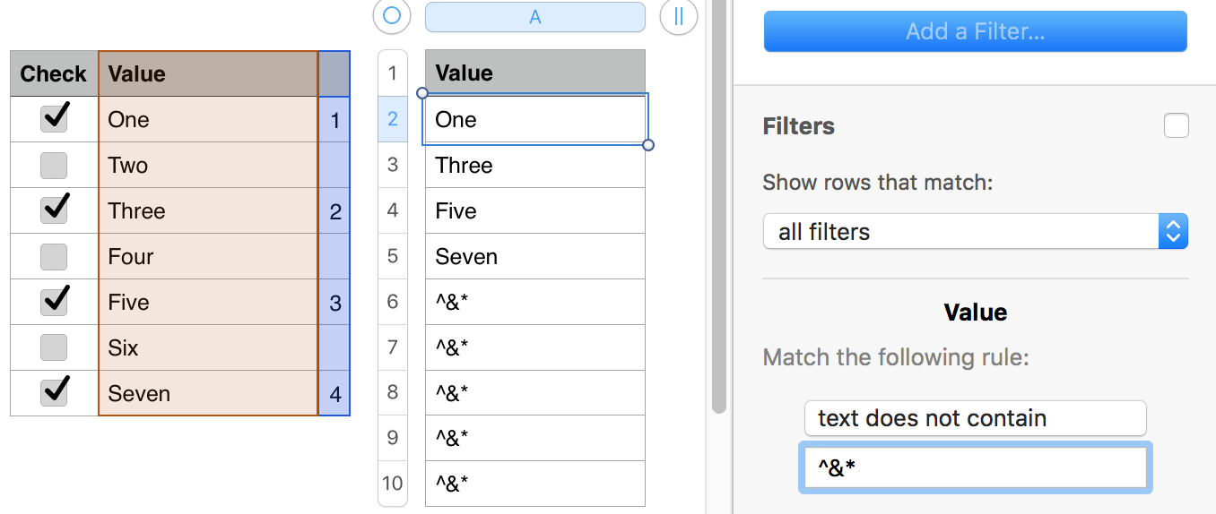
The ^&* string is there as a flag to a filter rule set to show only the cells that do not contain this three character string.

Hee are both tables, with the filter rule shown beside them, but not yet activated.

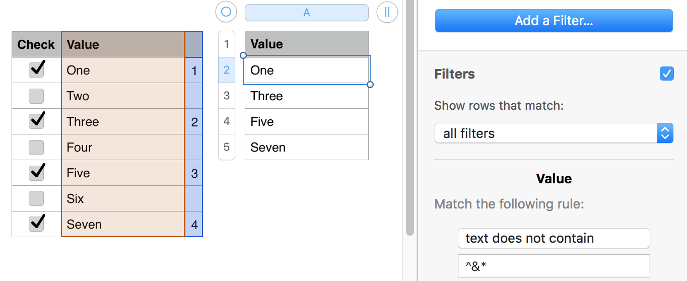
Clicking the checkox to the right of "Filters" checks the box and turns the filter on, with this result:

Regards,

Barry

Is there a reason you must have the results in a different table? (Note that "sheets" in Numbers have a blank canvas on which you place objects, including tables, so I think you mean table instead of sheet).

A filter is much the fastest way to do what you describe.

If you need the results in a separate table then just select the visible cells in the filtered table, command-c to copy, click once in a cell in an existing destination table (create one first if you don't have one already), and command-v to paste.

When you are finished and want to see the entire table again you can "turn off" the filter in Organize > Filter .

SG

Barry provides the answer to your question.

Somewhat easier perhaps: replacing the INDEX/MATCH pair of formulas with only one formula: XLOOKUP.

Something like this:

And replacing the "^&*" with the NO ENTRY symbol ⛔️ (or any other symbol, which can be filtered out).

Paul.

Skriddo wrote:

The tables are separate because the results will be printable, whereas the selection sheet(s) will not.

In that case a quick-copy paste word well. As described above:

"If you need the results in a separate table then just select the visible cells in the filtered table, command-c to copy, click once in a cell in an existing destination table (create one first if you don't have one already), and command-v to paste."

That only takes a second or so. Unless you have to do this often (every minute or so) then the filter approach is much faster and easier than setting up extra columns and entering formulas.

SG