What you are doing (mixing data up like this) is rather odd but here is a way to do it that is simple. I am showing it with the filter off. When the filter is on, all the empty rows in Table 3 will be hidden.
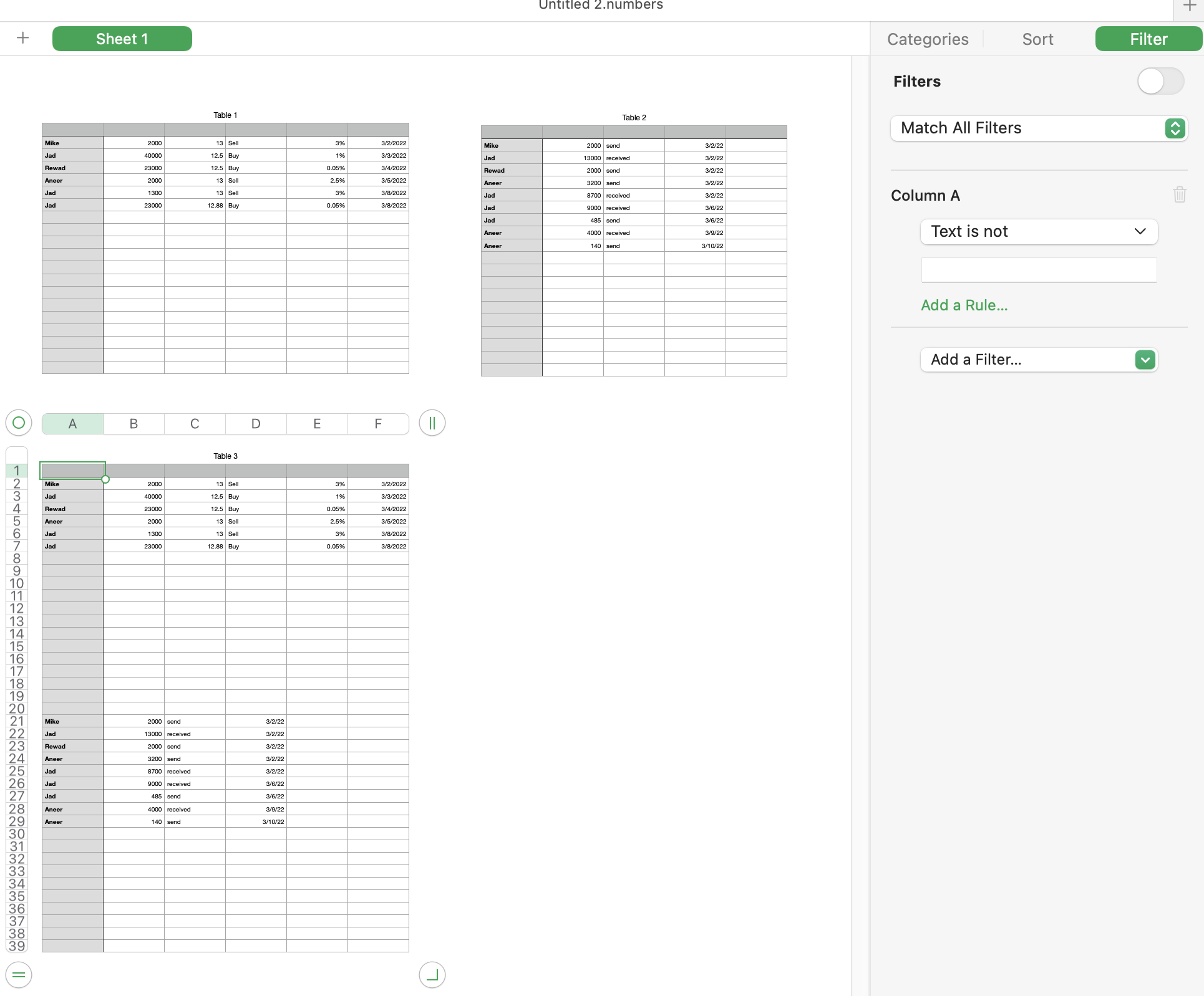
Table 3 is two parts. The top half brings in Table 1, the bottom half brings in Table 2.
Give Tables 1 and 2 as many rows as you think they will ever need. I used 20 rows for the example. Give table 3 the number of rows to fit both Table 1 and Table 2. This was 39 rows for the example. You cannot add new rows to Table 1 or 2 at a later time without remaking Table 3.
Formula in cell A2 =IF(Table 1::A2≠"",Table 1::A2," ")
Copy/paste down to row 20 and into B2 through F20 to complete the top half of the table
Formula in cell A21 =IF(Table 2::A2≠"",Table 2::A2," ")
Copy/paste down to row 20 and into B21 through E39 (not F39) to complete the bottom half of the table
The filter is "show rows where column A text is not a space character". You cannot see the space character in the filter but it is there. When the filter is on, you will see only the rows where a name appears in column A.
You can sort Table 3 to gather names together. This shuffles the formulas around, which will make a mess of the table in that respect. Just remember that there is no provision to sort it back to its original condition (other than using UNDO). You can add an additional column and put index numbers in it (1,2,3, etc as actual numbers not formulas) so you can sort back to the original state.
Be careful how you edit Tables 1 and 2. You can type data, you can copy/paste data, you can drag-fill data but do not select a cell and drag it to a new location in the table. That relocates the cell and the formula in Table 3 that references it will adjust to follow that cell to its new location, which is not what you want. And you cannot add new rows to Tables 1 or 2 without remaking Table 3.