Index and Match with arrays

That doesn't look like Number for Mac.

In any case, as you have discovered, Numbers does not support most "array formulas."

The easiest way is to use the built-in filtering functionality, something like this:

The formula in C2, of the extra column is:

A2=Search::$A$2

Then set a filter like this:

Then hide the filter column if you want:

Another quick approach is to use a Pivot Table.

Click in the data table and from the menu choose Organize > Create Pivot Table > On Current Sheet.

Then in the Pivot Option pane at the right drag fields from the 'Fields' box down into the 'Rows' and 'Values' boxes as shown, giving you something like this:

Control-click the amount for the Text value of interest and choose Create Table for Source Data.

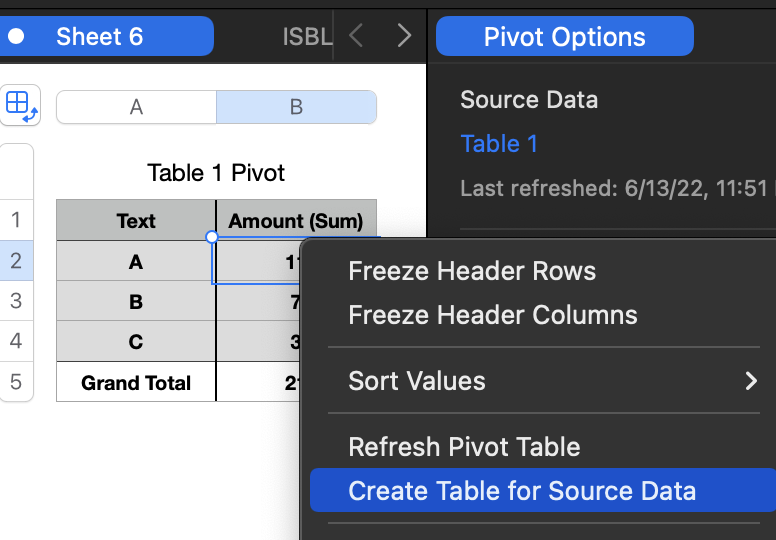
Giving you this:

Either way should be quick and easy, faster than reading this explanation.

SG

Hi Perry,

Here an alternative to Filter and Pivot Table

You would need an additional column for the counter in Table 1

You check if the search text was found and the count the number of matches up to this row.

Formula for cell C2: =IF(A2=Table 2::A$2,COUNTIF(A$2:A2,"="&Table 2::A$2),"")

In the result table you perform an XLOOKUP based on the current row number and counter.

Formula for cell A2: =XLOOKUP(ROW()−1,Table 1::C,Table 1::B,"",0,-1)

You can hide the column C after you tested everything.

Based on your region the , or the ; will be used to separate the different sections of a formula.

Hope this will solve your question, please let me know if something in unclear.

Ralf

Maybe something simple that is automatic (no need to refresh a pivot table) and keeps the same idea as the original with the results in a separate table:

Table 3 is as long as or longer than Table 1. My Table 3 is longer, causing error triangles for invalid references.

Formula in Table 3 cell A2 =IF(Table 1::B=Table 2::$A$2,Table 1::C,"")

Fill down to complete the column

The filter for the table is shown but is not turned on in the screenshot above

Below is the result with the filter on

The results cannot be sorted, they are in the order of appearance in Table 1 and will remain that way no matter how you try to sort it. I think that is how the Excel formula would work, too.

Here is one other way to do it with formulas:

Numbers: Function that returns many relia… - Apple Community

A choice among one simple formula using the built-in filtering functionality, a point-and-click approach with no formulas, and now an approach with two complicated formulas that we used to have to use before the new functionality was built into Numbers!

SG

PASEL wrote:

The sources tables are very big and I was getting tired of scrolling through thousands of rows looking for one line or keyword.

I will try the first example, but I haven't got pivot tables yet -

Ah, I see. Large tables can get a little cumbersome in Numbers. If your version supports Filters then that first approach may save you some work.

SG