Creating a formula if cell contains numbers that are +/- another cell

HI Hayley,

You wrote:

"What I am trying to achieve is to 'flag' the cell under DIFF. if it is either plus or minus more than the TOL. For example, looking at row 3, if the difference was either more or less than 1.25 it could be highlighted in some way, not necessarily a colour, but some other clever way to say this measurement is not within tolerance and is not acceptable. This would be my ultimate solution."

Isn't that precisely what is done in this example, copied from my third post above?

The red fill highlight in cells E4 and E5 says "this measurement is not within tolerance and is not acceptable."

"If … you need two columns, one with negative tolerance, and one with positive…

The "diff" column (labeled +/- in this example) includes minus signs where the spec value is less than the measured value and shows an unsigned (positive) value where the spec value is greater than the measured value. Is that distinction necessary, or would is it sufficient to know that the measurements for points B and C are both off-spec by 2 units?

If you do not need to distinguish between 'too long' and 'too short' in the diff column, then reporting the negative values as absolute (non-signed) values would remove the need for a second column containing the -TOL values.

If you do need the minus signs in "diff", then the -TOL column is needed (but does not need to be visible to the user).

, how do you create a rule to put a negative sign in-front of the tolerance? The form that pull the tolerance from only has the number with the title -/+. It's not viable to manually add a negative sign in front of the negative tolerance column (F3)."

(Note: In my example above, column F contains the (positive and unsigned) TOL value retrieved from the 'spec data entry' table. Multiplying this value by -1 converts it to the negative equivalent.

In the example posted here, the formula in G3 (and filled down) would be F3*-1

As you enter the formula, Numbers will automatically convert the apostrophe (*) to a multiplication sign ( × ).

As the results are negative, Numbers will automatically place the - sign.

As noted above, the -TOL column is needed by the CH rule, but does not need to be seen by the user in the usual course of business. Hide the column, or move it to the far right side of the table (and hide it there) to keep it away from the active part of the table, where it might be damaged.

Regards,

Barry

Regarding your second question:

"The other question I have, which should be a simple one, but I never know how to do it is, how do I copy the formula from point A to Z without manually entering it every cell? I also want to do the same thng horizontally across."

There are a couple of ways to do this more efficiently.

1. Enter the formula in the first cell in which it is needed.
2. After pressing enter, hover the pointer near the bottom of the cell containing the formula.
3. When the Fill control (a small, yellow filled circle) appears in the bottom boundary of the cell,

     place the pointer on that control, press and hold the mouse button, then drag down the column to fill the formula into the rest

    of the cells requiring it.

Each of the cells in the column will now contain a copy of the formula. Row numbers of cell references in the formula will have been incremented by one row to keep the same relative position wrt the cell that copy is in.

Filing across a row:

Same as above, but the Fill control will appear on the side of the initial cell in the direction you will be dragging, and the Column references will increment as the formula is filled into new columns.

For long column fills:

1. Enter the formula in the first cell.
2. Select that cell, and press command-C to copy the cell (and its formula).
3. With the first cell still selected, scroll to the last cell in the column that is to receive the formula.
4. Press and hold the mouse button, and click on the 'last cell' to add it and all cells between it and to the selection.
5. Press command-V to paste the formula into all of these cells.

Done.

Regards,

Barry

Hi Hayley,

You wrote:

" I am wanting to create a formula that will highlight a number if the TOL. higher or lower than the number in the +/- cell."

The formula shown in your example is entered in cell F3 of the main table in your example.

This formula gets the value ("A") from cell A3 o this table, searches for that value in column C of the table SDEntry, and if that value is found, returns the value from the cell in the same row of column F of that table.

If the value is NOT found, the formula returns a null string ( "" ), a text value with zero length.

The formula is enclosed in an IFERROR statement, which returns a null string if the core XLOOKUP formula returns an error.

Question: What errors are you expecting to occur?

"I am unable to use a conditional format as there is already a formula in that cell dragging a number from another page."

Conditional Highlighting does not depend on formulas. It is controlled by a set of one or more rules that compare the value to be highlighted with a fixed value, written into the rule, or with a variable value determined in a different cell.

In your example, TOL is a positive value, while the +/- value in E3 is determined by subtracting the measured value from the specified value'.

If the difference between the measured value and the spec value is less than or equal to the TOL value, the measured value is 'within tolerance', and the highlight should consist of a 'green light.

The difficulty in comparing the two values is that you are comparing a positive value (TOL) with another value that may be

greater than that positive value (not within tolerance),

less than that positive value, but still positive (within tolerance),

less than zero, but not as far from zero as TOL (in tolerance)

or less than zero and further from zero than TOL (not within tolerance)

The easiest way to compare those values is to convert the +/- value to an ABSolute value, then do the comparison as I've done here:

Column F in this example contains a formula that converts the +/- value in column E to an absolute value which is used only to determine the highlighting in the TOL column. This column does not need to be seen in your table, nor does it need to be placed where it is. This (and the equivalent 'compare value' column for each of the other TOL::+/- comparisons can be added to the right end of the table, then hidden from view.

Regards,

Barry

Hi Hayley,

The rules for conditional highlighting aren't as flexible as you'd like them to be.

Each rule compares the value to be highlighted with a single other value. That other value can be written into the rule, or can be placed in a cell using a formula.

The value in a single cell may be tested with several rules. If that is done, the order in which the rules are listed is usually significant. The rules are tested individually, starting with the first in the list. If the first test returns false, Numbers moves on to the next rule, and continues until either it runs out of rules for that cell, or it comes to a rule that returns true.

You want to highlight the value in E3, which is the difference between the specified value and the measured value. If this difference is greater than the maximum tolerated deviation above the specified value OR less than the maximum tolerated deviation below the specified value you want to highlight this cell.

Each cell to be highlighted will need to be tests against two values: the maximum tolerated deviation above the specified value (+1.25) and the maximum tolerated valued below the specified value (-1.25). If the deviation is further from the tolerated deviation in either direction, the cell containing that deviation value is to be highlighted, otherwise, no highlighting is to be applied.

The tests will require a comparison with the values in two cells, one containing the positive deviation limit, the other containing the negative deviation limit. If either test returns true, the tested cell is to be highlighted; if both return false, the cell is t be left unhighlighted.

Here is an example:

Column F contains the TOL values as a positive number.

G3 contains the formula F3*-1, filled down to the end of that column.

Select all cells containing a +/- value in column E, then construct the two conditional highlighting rules as the would apply to cell E3. Numbers will automatically increment the row numbers to match the row in which the rule is placed for each cell in column E.

To enter individual cell addresses is the second row of each rule, click the icon (not shown in the example) at the right end of the second box in the rule, then, in the Table, click the cell (F3 in Rule 1, G3 in Rule 2) whose address is to be placed in that box.

As noted earlier, 'column G' can be placed elsewhere in the table, and can be hidden, if needed.

Regards,

Barry

" Am I able to add something in front of my formula to automatically add a - (negative) in cell F and a + in cell G?"

Why?

TOL is a non-signed value, stating how close to the specified datum the measured value must be to be within the specified tolerance. The negative values in column G of my example are there only to give the second Conditional Highlighting Rule a value it can test to determine if the the measured value is less than the minimum value within the tolerance range. The value must be available to the Rule, but does not need to be visible to the user.

Here are two screenshots of the same table (with several added columns to represent the repeated 'Spec' to 'Amended Spec' sets in your example.

The first one shows the 'column G' of my example moved to a new location to become 'column Z'.

In the second image, below, column Z has been hidden, as there is no need for the user to see it. Hiding it does not affect the ability of formulas or CH Rules to use the values in that column, though, so again, there is no change in the result displayed in column E.

Numbers has automatically revised the formula and the CH rules to fit the new location, so there's no change in the data displayed or the conditional highlighting of the cells in column E.

Regards,

Barry

"I would like to know how I work out the average percentage out of tolerance, either above or below."

EDIT: After going through the calculations on the first part here, I'm not sure my first section is calculating the values you are looking for. Can you provide a more precise description of what you consider the "average percentage out of tolerance" to mean?

Meantime, a quick look at the formulas in the first part, using values from your table above, may be useful.

B.

Part 1:

This would be the average of the 'distance' from the specified values.

To calculate that average, you'll need to sum the absolute values, then divide be the count of those values

Here's an example:

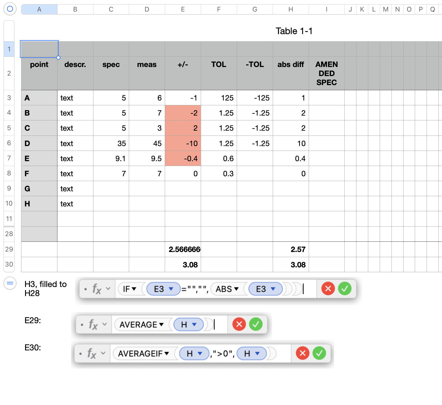
The first formula, entered in H3 and filled down to the row (28) above which the averages are to be reported. The formula strips the signs from the values in column E and places the signless value in the same row of column H.

Rows 29 and 30 are the bottom two rows of the table, and have been converted to Footer Rows. A table may have up to 5 Footer rows, but they have to be contiguous and the five (or fewer) at the bottom of the table.

Using a footer row allows clicking the column reference tab to choose all of column H without including the Header or Footer rows.

The difference between the two formulas is that AVERAGE will ignore cells containing containing text, but will include cells containing zero, while AVERAGEIF (as written) will include only cells containing a value greater than zero in its Average calculation.

Both formulas were entered in the same rows of column E and column H. The results in column E are the results calculated by each of the formulas; the displays of the same results in column H have been rounded to two places after the decimal for easier reading. Rounding the display does not change the actual value placed in the cell.

Part 2

Following that formula I would like to say "if tolerance outside 10%, the garment is not acceptable."

Not sure what your message is here, or what "outside 10%" refers to.

"Tolerance," to my understanding is a statement of the maximum difference from the specified quantity that is acceptable (ie. 'that will be tolerated').

"10%" is a fraction (n/100) presented as the numerator with the denominator set to 100.

10% is equivalent to 10 hundredths or 1 tenth.

My questions here is 'one tenth of what?'

Does this apply to a single measurement, or to the average of all measurements?

Four of the points on your list show a tolerance of (plus or minus) 1.25 units.

The fifth point shows a tolerance of 0.6 units.

The sixth point shows a tolerance of 0.3 units.

How is the "10%" to be calculated for these three cases?

Regards,

Barry

Your IFS formula is missing a final condition-result pair.

The last pair requires a pair in which the condition always returns 'true' and the result if true tells Numbers what to do if none of the 'real' conditions were met. In this case, neither the first (less than or equal to -3) nor the second (>3) were met, so the formula had to look for the next pair, which isn' there yet.

Editing the formula in your most recent post to include the required pair would look like this:

IFS(I29<-3,"NO",I29>3,"NO",true,"Yes")

That said, here's a different approach using IF and ABS:

ABS changes the negative values to 'absolute' (signless) values and makes no change to positive values or to zero.

IF compares the result with the (positive) value 3 and returns "Yes" if that value is less than or equal to 3 or "No" if that value is more than 3.

The Column part of the cell address (I29) changes as the formula is filled right into columns J to O to match the column containing that copy of trhe formula.

Regards, Barry

"What about if there is not entry. How do get the cell to remain empty."

I've usually added an IF statement to act as a 'switch' to bypass the formula if there's no entry in the 'trigger cell'.

Core formula: IF(ABS(B3)≤3,"Yes","NO")

Switch added: IF(B3="","",IF(ABS(B3)≤3,"Yes","NO"))

Regards,

Barry