Rank Values Based on Multiple Criteria

Hi Bear34_1,

as you have learned RANK can only check for one criteria, therefore you have to calculate a new criteria that will combine your two existing criteria.

Here one possible solution:

It will work as long as the sum in the column B, E, H, K, and N will stay below 1,000 and you have max 9 groups of columns.

Row 7 is a simple copy of the count for the checkmarks in row 5, this will make the RANK formula in row 8 easier.

Formula for A8=RANK(A7,$A7:$N7,largest-is-high) $-signs are important to preserve the columns

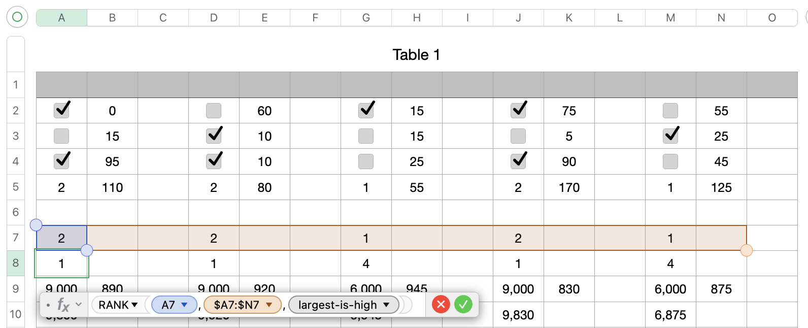
Formula for A9=10000−(A8×1000) Here I will calculate a support value.

If the rank is 1 I get 9000, if it would be 2 I get 8000, ... This will ensure that a high rank will get a high total value.

Formula for B9=1000−B5 Here I will calculate a support value.

If the total from B2 to B4 is low I get a high result

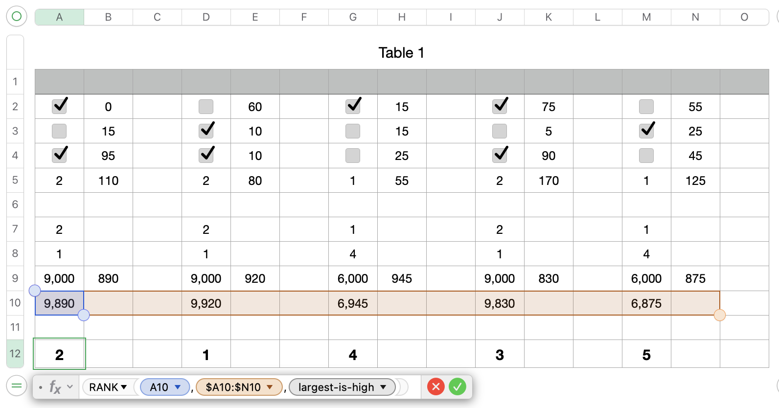
In A10 I create the sum of A9+B9

Formula for A12=RANK(A10,$A10:$N10,largest-is-high)

This will give you the rank based on the calculation for the support values.

You can hide rows 6 to 11, to have a clean looking table.

Based on your region the , or the ; will be used to separate the different sections of a formula. If you write one thousand as 1,000.00 then the , is used as your formula separator. If you write one thousand as 1.000,00 then the ; is used as your formula separator.

Hope this will solve your question, please let me know if this worked for you or if something in unclear.

Regards Ralf

Another solution would be this:

A6 = A5+1÷(B5+2)

copy/paste to D6 etc

I added 2 to B5 so that the max value the decimal part can ever be is 0.5, never as large as 1. The assumes that the values in columns B, E, etc are positive values.

A7 =RANK(A6,6:6)

copy/paste to D7, etc.

Hi Bear34_1,

could you please check your description and your attached screenshot.

Based on how I understand they do not macht!

A, D, G, J, and M are TRUE as soon as they have a checkmark.

Column J is the only one that has 3 TRUE checkmarks, therefore it should be 1st.

The columns with 2 TRUE checkmarks should be 2 and 3.

The columns with 1 TRUE checkmarks should be 4 and 5.

What range would the columns B, E, H, K, and N have?

0 to 100, 0 to 1000, or something other?

I assume that you would like to rank based on the totals in row 4, correct?

I added the ranking in yellow, based on how I understand it.

Regards Ralf