A COUNTIF() formula on each of the tables should do the job. You will be able to highlight the cells containing the formula, not the one containing the original item name. Here's a simple example.
 The table on the left is named "Then", the one on the right is named "Now". The formulas in each table, entered in cell B2, then Filled down the rest of the column, are identical, except for the Table name in the cell reference to column A of the other table:
Then, B2: =COUNTIF(Now :: $A,A2)
Now, B2: =COUNTIF(Then :: $A,A2)
The conditional formatting rule for column B sets the same condition, but a different colour fill. Conditional formatting rules are set through the (Cell Format) Inspector.
Here's a second example, with a more complex formula that provides two enhancements:
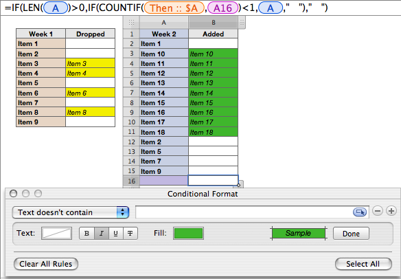
- Note that the selected cell (B16) is no longer highlighted. This is handled by the first IF statement, which tests ( LEN(A)>0 ) for an entry in column A, and inserts three spaces into its cell if no entry is found.
- If an entry is found, the formula counts the occurrences of that entry in the other table. If the count is zero, the formula copies the item name from column A into its cell in column B; if the count is greater than zero (ie. if it is 1, assuming no double entries), the formula places a string of three spaces in its cell.
The revised formula looks for three consecutive spaces in the cell. If these are not found, the rule applies the selected highlight colour.
The two tables could be constructed each week, but it would be simpler to save the document as a template, then each week paste the item names from the previous week into the "Then" table and the new list into the "Now" table.
Regards,
Barry