Last column value

TR,

Here's a simple implementation:

=OFFSET(B1, COUNT(B), 0) is the formula in the Footer Row cell displaying the last value.

Curious how you did it in Excel. Same method should work in Numbers, I would think.

Regards,

Jerry

you can determine how many rows there are in a column by using the function ROWS(). You can then use the offset() function to retrieve the value using the rows() function.

something like:

in the table on the left:

A1=OFFSET(Data Table :: $A$1, ROWS(Data Table :: A)-1, 0)

The table on the right contains the column you "regularly" update.

I hope this helps

trexo,

I provided a formula. Can you provide any context as to specifically what you are trying to do OR the Excel formula you are using?

Wayne

trexo,

you have to name the tables the same as I did... the right table was titled "Data Table". If your table is not named that AND you copied the formula I posted you will get the error your reported because the table you are attempting reference, in fact, does not exist so the reference is invalid.

This will work better for you-- I hope 😉

B4=OFFSET($D$7, ROWS(D)-7, 0)

Wayne

trexo wrote:

Thank you Jerrold for your reply. I have seen your similar posts and have tried the offset command. Does the formula have to be in the footer? I am not familiar with putting formulas in footers. All my data is in column d. I would like the value to appear in cell B4. In converting my spreadsheets from excel to numbers this formula did not translate well. In excel I used the following:

=index(D:D, Match(9.9999999999999E+307,D:D))

That formula put the last value in column D into whatever cell I put the formula.

Yikes, I can see why you weren't excited about using that formula. You can put that formula of mine anywhere you wish. I'm making the assumption that you would be capable of adjusting the formula for the actual location of your data. Header and Footer rows are handy tools for isolating the data from the labels and summaries. Crack open the Numbers User Guide and become familiar with some of the interesting features in Numbers that make life easier than with Excel. Headers and Footers are quite useful.

Jerry

trexo,

Jerry and I both presented solutions but now, after looking at Jerry's solution, I am not sure which one is the one you are looking for... the distinction is that Jerry's will return the last value from a column even if it is not in the last cell of the column. Mine will only return the value in the last actual cell of the column. My guess is that Jerry's solution is the one you want since it is more general-- that is if the last cell in the column is filled our formulas will both work.

Wayne

Hi trexo,

Jerry's original solution, reproduced here, may be placed in any cell on the same table as the list of values in column B.

=OFFSET(B1, COUNT(B), 0)

It assumes that the first value in the list is in cell B2 (one row below the label in Row 1), and that (as you specified) there are no gaps in the data from that cell to the last one containing a value.

COUNT(B) counts the numerical values entered in column B; the result is used as the row-offset in the OFFSET function. Zero ( 0 ), the column-offset value in the formula, means 'the same column as the base, B1'.

Your Excel formula:

=index(D:D, Match(9.9999999999999E+307,D:D))

MATCH returns the position of the specified value in a list of values in a range.

The range here is column D, and the value to match (expressed as a base 10 number) is

99999999999999 followed by 294 zeroes, a rather large number, likely to be far greater than the largest number in column D.

MATCH in numbers can be set to find the largest close match, the smallest close match, or an exact match, with 'largest close match' the default choice. My assumption is that this is also true in Excel. If so, the expression in your Excel formula is looking for the "largest number in column D that is smaller than or equal to the search value."

IF the last number in the column is also the largest number in the column (and that number is smaller than 9.9999999999999E+307), then the formula will return the correct value. If the last value in column D is NOT also the largest value in column D, OR is larger than the search value, then the formula will not return the 'last value' in column D.

A Numbers similar to this would be:

=OFFSET(D1,MATCH(9.9999999999999E+307,$D)-1,0)

Here's an example, showing the results. The formula above is in B2; the same formula with the cell references changed to E1 and $E is in B3:

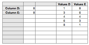
Note that both return the largest value in their column, not necessarily the 'last' value in that column.

Regards,

Barry

What is in the last cell of the column? If that cell is empty then the formula will return "0"

Trexo,

If my solution doesn't work for you, I'm curious why that is the case. Could you please describe what you expect, and what happened when you tried my solution.

Kind regards

Jerry

Trexo,

Wayne's formula gives you the value in the last row of the table. It sounds to me like you want the last value in the column, not the value in the last row of the table. This is why you are getting a result of "0", you have nothing entered in the last row. You need Jerrry's solution. And, yes, it works on the iPad.

Turning off what you are calling "autocomplete" would make formulas harder to construct on the iPad. It is great the way it is.

That Excel formula is a mess. It uses a design flaw in the MATCH function in Excel to do its work. MATCH is supposed to be finding the largest value less than or equal to 9.999E307. In other words it should find the largest value in the column, not the last value in the column. The formula works as it is supposed to in Numbers.