Hi Elissa,
This looks like a classic LOOKUP situation.
Here's a skeleton view of the three tables involved.
Table 1 is your input table, with values selected in B3 and C3.
Panels is your orange-striped table, with location labels (eg. C4) used in lieu of re-typing the actual data.
Table 4 represents a set of cells in your Table 4, into which the requested data is rtransferred.
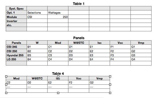
Panels is treated as a Lookup table, with the identifiers in column A as the search values.
Table 4::A2 contains the formula below:
=VLOOKUP(Table 1 :: $B3&" "&Table 1 :: $C3,Panels :: $A:$G,COLUMN()+2,0)
Syntax: VLOOKUP(search-for,search-where,result-column,match type)
Table 1 :: $B3&" "&Table 1 :: $C3 constructs the search-for string by concatenating the contents of Table 1::B3, a single space, and the contents of Table 1::C3. Result: "CSI 255"
Panels :: $A:$G tell Numbers the lookup table is columns a through G of Panels, Numbers searches for "CSI 255" in the firt column of the Lookup table.
COLUMN()+2 COLUMN() returns the number of the column containing the formula (1), +2 adds 2 to this value to tell the formula to return the value from the third column of the Lookup table (column C). As the formula is filled right, the result of Column increases, and the formula continues to return results from thecorrect column.
0 (or FALSE) means don't accept a 'close-match. If the exact search-for value is not found, the formula will return an error message.
To use the eror message, the whole formula is enclosed in and IFERROR statement:
=IFERROR(VLOOKUP(Table 1 :: $B3&" "&Table 1 :: $C3,Panels :: $A:$G,COLUMN()+2,0),"---")
The results of this version may be seen in Row 3 of Table 4, where the formula is looking for the values in B4 and C4 of Table 1.
Regards,
Barry