How do I match a result to the color of certain cells?

Hi Michael,

Let's start by moving the screen shot into this thread, where it can be seen and referred to without having to flip between pages in the browser:

Formulas cannot detect the colour of the fill in a cell.

But you could approach it from a different direction: Cell fill colour can be set by rules that compare the value in a cell with a fixed value or the value in another cell.

Similar conditions, can be used in a SUMIF or SUMIFS based formula to determine which numbers are included in a sum.

What rule do you follow to determine the background colour of the name cell? Could you use a checkbox to dictate that change? Or a popup menu?

What is the purpose of the checkboxes in column C? When do they get checked?

More details on the overall problem, please.

Regards,

Barry

Michaël,

Short of an Applescript solution written by one of the forum's experts like Hiroto, you're best approach would be to manually tick a checkbox in a new auxiliary column for every green confirmation signal. The checkbox can then be used in a formula.

Unless you have thousands of these cases, the manual approach would be the quickest.

Jerry

Hi Michael,

Jerry's suggestion is more or less where I was going as well.

Here's an example, with the checkbox placed in a (new) column A, and conditional formatting applied to the cells in column A, using the rule shown below the table. Default fill colour for column A has been set to the 'salmon' shade shown.

The next step gives the appearance of colouring the whole row for each checkbox checked. It uses an auxiliary table that copies the value from each row of column A, then applies a similar conditional formatting rule. Here the two tables are shown separately. Note that the CF rule also sets the text colour to the same green hue as the fill.

The final steps are to set Fill in the main table to 'none' (white square with diagonal red slash), then move the auxiliary table to the back, then slide it under the main table, allowing the colours to show through. I've added some text to the main table before doing this, so the effect can be seen.

Regards,

Barry

Hello

Barry has already shown the authentic way of doing this in Numbers.

Here's another way using AppleScript although you need to run the script manually when you update the table, which is the major drawback.

To use this, copy the code lised below in new document of /Applications/Utilities/AppleScript Editor.app and run it. The script will pick the colour to be totalled from the last cell in column B and calculate the total as described. (You need to set the fill colour of the last cell in column B, which is supposed to be the cell for the total, to the green colour.)

(*
    The sum cell S = the last cell of column B
    The sum colour G = the fill color of S
    The value of S = (unit) * (count of rows in column B whose fill colour is G)
*)
_main()
on _main()
    set unit to 63.45 -- unit price
    
    tell application "Numbers"
        tell document 1's sheet 1's table 1
            tell column 2
                set bg to cell -1's background color
                set n to count (cells whose background color = bg)
                set cell -1's value to unit * n
            end tell
        end tell
    end tell
end _main

Hope this may be of some help,

H

Oops. The previous script counts the cell for the total itself and adds extra one. Sorry. Corrected code follows.

(*
    The sum cell S = the last cell of column B
    The sum colour G = the fill color of S
    The value of S = (unit) * ((count of rows in column B whose fill colour is G) - 1)
*)
_main()
on _main()
    set unit to 63.45 -- unit price

    tell application "Numbers"
        tell document 1's sheet 1's table 1
            tell column 2
                set bg to cell -1's background color
                set n to count (cells whose background color = bg)
                set cell -1's value to unit * (n - 1)
            end tell
        end tell
    end tell
end _main

All the best,

H

Hi Michael,

The content of B2 ( "BBB" in my last image) has no effect on the fill colour of that cell. The original table has it's fill colour set to 'none', making the table and all of its cells transparent.Here's the original table again, this time with the fill colour and conditionally set fill colour removed from column A, and with an oval shape, filled with a colour gradient placed behind it. Note that the shape can be seen through all cells except those in the Header Row (1) and the Footer Row (11).

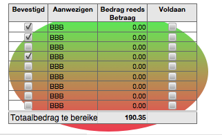
The colours are the result of a fill colour (salmon) and a conditional fill colour (green) applied to a second table. In practice, text in the second table is given the same default colour as the fill colour and the same conditional colour as the conditional fill colour. For this illustration below, I've chosen hues that are slightly different to permit seeing the text in each of these cells. Here is the same table shown above, with the oval shape taken away, and the second table shown below the original:

Note that the second table is a single column table, has a Header row, but no footer row, is the same width as the original table, and has rows that are the same height as the corresponding rows in the original table.

The formula on this table, entered into cell A2, and filled down to A10, is shown below:

A2: =Table 1 :: A2

Each cell corresponding to a checked box contains "TRUE"; each corresponding to an unchecked box contains "FALSE".

The Conditional format rule (shown in my post above) sets the fill and text colour to green if the cell contains "TRUE".

When the second table is placed behind the original, the colours show through, and the rows appear to be coloured.

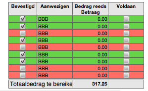
Note that two more people have now confirmed, their rows are coloured, and the total has increased.

The total is calculated in cell C11 by counting the checked ("TRUE" boxes, and multiplying the price per person by that count:

C11: =63.45*COUNTIF($A,TRUE)

Regards,

Barry