I need help calculating the "occupancy rate" of a lodge.

I would really like to help with this but might need some more info. first if you could clarify for those of us not in the rental or hotel business, how is "occupancy rate" calcuated by hand?

Second, if you could actaully hide the columns in your screen shot instead of blurring them out. Blurring them just seems to makes it harder to see when it shows in the limited zoom window.

Offhand, if % occupancy is as simple as (number of days occupied)/30 then you can have a summary table that has date range versus Cabin number. Use sumifs to add up your column of days per cabin. divide by the date difference between start and end dates. plot that.

Jason

Caleb,

Thanks for making your data available. The first thing I noticed is that you have some data entry errors in the dates. It isn't apparent when you use the short year form, but some of your dates are in the years 0012 and 0013, 2000 years ago. Sorting that out will improve the calculations. 🙂

Jerry

Caleb,

Here's a simple calculation, not exactly what you wanted, but much easier to achieve.

In the summary table I used a SUMIF function to find the total days booked for each unit, and for the total days available, I subtracted the earliest check-in date from the latest check-out date.

Jerry

Caleb,

In my summary table, the expression for Days Occupied is:

=SUMIF(Accepted Bookings :: C, A, Accepted Bookings :: G)

The expression for Rate of Occ is:

=B/$B$8

I'd like to help you with the breakdown by month, but it's not an easy putt. There was an almost identical question here in the past 12-18 months - you can probably find the discussion if you have some luck searching. I recall working on the solution and finding it quite complex. I don't think it's worth the effort in your case considering how sparse the data is, but that's your decision. You will be using SUMIFS (note the extra "S") to further constrain the summations to a particular month. But, the main issue is the problamatic reservation that spans the end of month; difficult, as you have speculated.

Good luck,

Jerry

Hi Caleb,

If I'm reading your table correctly, the unit numbers are i column C, In date in column E, Out date in column F and duration of stay in column G.

For stays that do not cross from one month to another, a simple SUMIFS statement woud work to calculate the number of occupied days in a given month. As you've found, theough, the stays that begn in one month and end in another are a bit trickier.

One way to resolve the issue is to use an auxiliary table which calculates the occuped days (for all units) using a separate column for each month, then a summary table to sum the monthly data for each unit.

Here's an example, using random data over a two and a half month span.

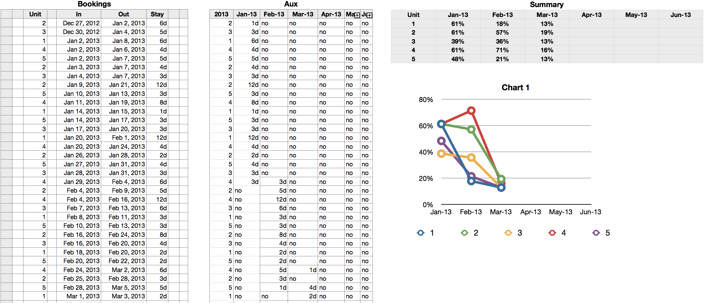
Note that the dates in the header row of Aux and Summary are actual Date and Time Values set to the first of each month, and formatted to show only the month and year. These are used in the calculations.

The only formula in Bookings is =F-E in each cell of column G (Stay).

Aux has two formulas:

A2, and filled down: =Bookings :: C2

This simpy copies the values from column C of Bookings to column A of Aux.

B2, and filled down and right:

=IF(AND(Bookings :: $E2>=B$1,Bookings :: $F2<EOMONTH(B$1,0)+1),Bookings :: $F2-Bookings :: $E2,IF(AND(Bookings :: $E2<B$1,Bookings :: $F2>B$1),Bookings :: $F2-B$1,IF(AND(Bookings :: $E2<=EOMONTH(B$1,0),Bookings :: $F2>EOMONTH(B$1,0)),EOMONTH(B$1,0)+1-Bookings :: $E2,"no")))

Same formula, separated into sections:

=

IF(AND(Bookings :: $E2>=B$1,Bookings :: $F2<EOMONTH(B$1,0)+1),Bookings :: $F2-Bookings :: $E2,

IF checks if the IN date AND the OUT Date are both in the month for this column. If so, the calculation is done and the formula is done; if not, control is passed to the next if:

IF(AND(Bookings :: $E2<B$1,Bookings :: $F2>B$1),Bookings :: $F2-B$1,

IF checks it the IN date is before the month for this column AND the OUT date is after the beginning of this month. If so,th calculaton is done and the formula is done; if not, contorl is passed to the thrid IF:

IF(AND(Bookings :: $E2<=EOMONTH(B$1,0),Bookings :: $F2>EOMONTH(B$1,0)),EOMONTH(B$1,0)+1-Bookings :: $E2,

IF checks if the IN Date is before the end of the month for this coumn AND the OUT date is after the end of the month. If so, the calculation is done; if not, the text blow is returned to the cell.

"no")))

This text was chosen to give me a visual indication of the result. In practice, I would replace it with the empty string ( "" ).

Summary has a single formula:

B2, and filled down and right:

=IFERROR(DUR2DAYS(SUMIF(Aux :: $A,$A2,Aux :: B))/DAY(EOMONTH(B$1,0)),"")

SUMIF sums the duatons of Stay for each unit in a specific month for each column.

DUR2DAYS converts the duration to a number of days.

DAY(EOMONTH(B$1,0) returns the number of days in the month whose date is in row 1.

The first is divided by the second, and the result is formatted as percentage, with 0 decimal places.

IFERROR traps the error that occurs when the source column on Aux contain only text values, and replaces the error message with the empty string.

Regards,

Barry

Hi Caleb,

Cell references without a table name attached refer to cells on the same table as the formula. B1, on the Summary table, contains the Date and Time value January 1, 2013 00:00:00, formatted to show only the (short form) month and year values, joined by a dash.

The $ operator holds that reference to row 1 as the formula is filled down the column. The lack of the $ operator before the B permits that column reference to change as the formula is filled to the right.

Regards,

Barry

PS: If you haven't yet done so, i'd strongly recommend downloding and reading at least the first four chapters of the Numbers '09 User Guide to learn some of the basics of working with Numbers. You'll find a link to the download in the Help menu in Numbers '09.

Also available in the same place is the iWork Formulas and Functions User Guide, in which you'll find descriptions and usage examples for all the functions available in Numbers.

B

Hi Barry,

I have a similar problem and I tried to replicate your solution, using the same tables, but I keep getting a wrong format error.

My Numbers is in Italian, so you will see some differences in the "AND", "IF" etc.. as they are translated. Still, I don't understand why your function doesn't work for me.

Please see the image attached. I copied and pasted in a text box the function you used as reference.

The B1 cell is an actual date (1/1/2013 00:00:00)

I would appreciate any help!

Thanks

Mauro

Hi Mauro,

I suspect the issue is that you are using the comma ( , ) as the argument separator in the formula, and the application, in locations where the comma is used as the decimal separator, expects a semi colon ( ; ).

Regards,

Barry