HI Peter,
I've been following this conversation off and on for the past few days, and have a few questions/comments.
Screen shots: Grab is OK, but I find the procedure described above by Ian simpler (and more famiiar, since it's been part of the Mac OS snce before Grab was even thought of). Here's a review:
- Make sure what you want a shot of is on the screen.
- Place the mouse pointer at one corner of the area you want to include in the shot.
- Press shift-command-4 (The mouse pointer will change to a crosshair.)
- Press and hold the mouse button; Drag a selection rectangle to enclose the area you waant in the shot.
- When the rectangle encloses your well-composed shot, release the mouse button.
The screen shot s now savd to your Desktop, with the title "Screen Shot..."followed by the date and time.
To post the sreen shot:
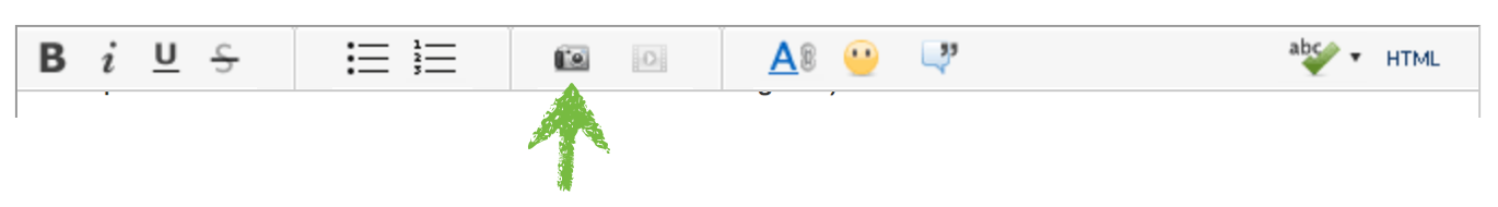
- Click the camera icon in the bar above the compose window:
- In the dialogue that opens, Click Choose File.
- Click the fine name in the Choose window. Click Choose.
- The Choose window cloes. Click Insert File.
(See Ian's note regarding having to repeat this procedure on the first attempt.)
Done.
Formulas:
"=IF(ISBLANK(A),"",IF(F3=TRUE,F3,VLOOKUP(E3,Index::A:WHO graph level,2,0)))"
F3 contains the result of a test for A3 being not blank. Since F3 will always be the opposite of the first IF's condition, this test is redundent, and can be romoved (as can the whole of column F).
Revised formula:
=IF(ISBLANK(A),"",VLOOKUP(E3,Index::A:WHO graph level,2,0))
OR
=IF(LEN(A)<1,"",VLOOKUP(E3,Index::A:WHO graph level,2,0))
OR
=IF(LEN(A)>0,VLOOKUP(E3,Index::A:WHO graph level,2,0),"")
"=IFERROR(NOT(ISBLANK(A)),)"
This is the formula in column F, and may be eliminated.
"=IF(F3=TRUE,AVERAGE(G$2:G3),"")"
With column F eliminated. this needs a simple replacement of the F3=TRUE test with the test that made F3 "TRUE"
=IF(LEN(A3)>0,AVERAGE(G$2:G3),"")
You mentioned that this formula "provide(d) a forward projection to the end of the current month," which it does not.
If you want it to repeat the last average to the end of the month, make this change:
=IF(LEN(A3)>0,AVERAGE(G$2:G3),G3)
While this will give you a stright line across th rest of the graph, the line is pretty meaningless. I would eliminate it as misleading.
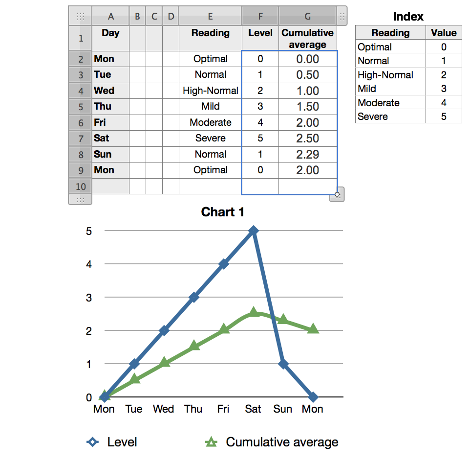
Here's the result, with a chart showing both daily values and the cumulative average to each day.
Regards,
Barry