Missing a Formula for ignoring blank cells.

Hi Tim,

Interesting question!

Here's a possible solution. It requires two auxiliary columns (which may and should be hidden) to be added to Table 1, and a new formula to count the draws in Table 1-1, column D:

Table 1:

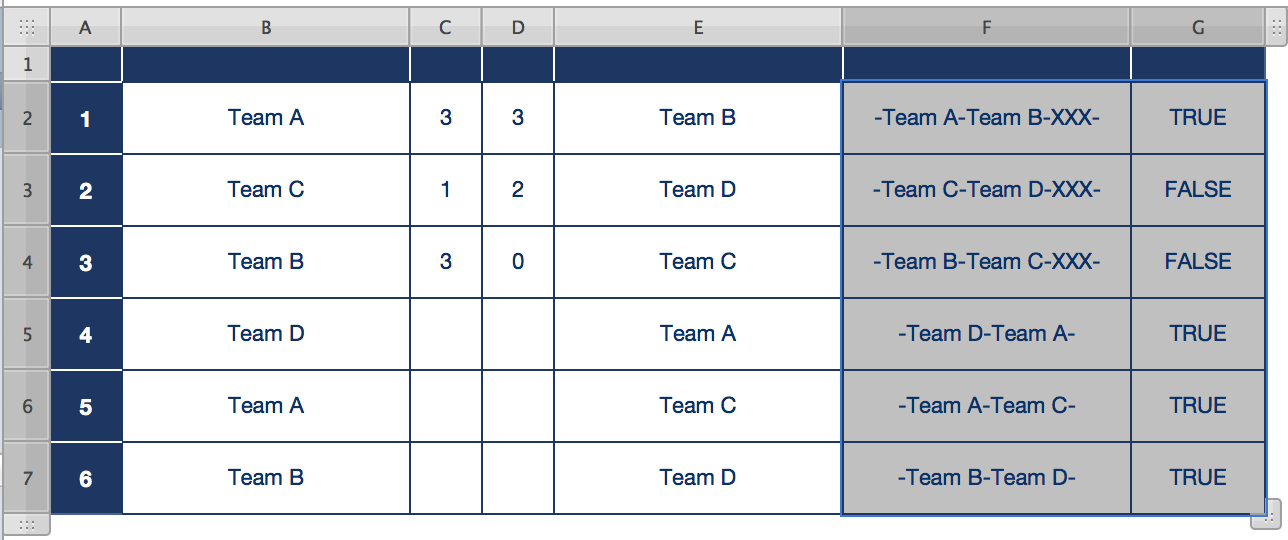
Columns F and G are the auxiliary columns. The formulas below are entered into row 2, then filled down to row 6.

F2: ="-"&B2&"-"&E2&"-"&IF(AND(LEN(C)>0,LEN(D)>0),"XXX-","")

This constructs a string consisting of the names of the opposing teams (from columns B and E) plus a code ( XXX ) that indicates scores have been entered for both teams (ie, the game has been played).

G2: =C=D

This returns TRUE if cells in column C and D have identical contents, and FALSE if their contents differ. TRUE indicates a possible draw, FALSE that one or the other team has won.

Table 1-1

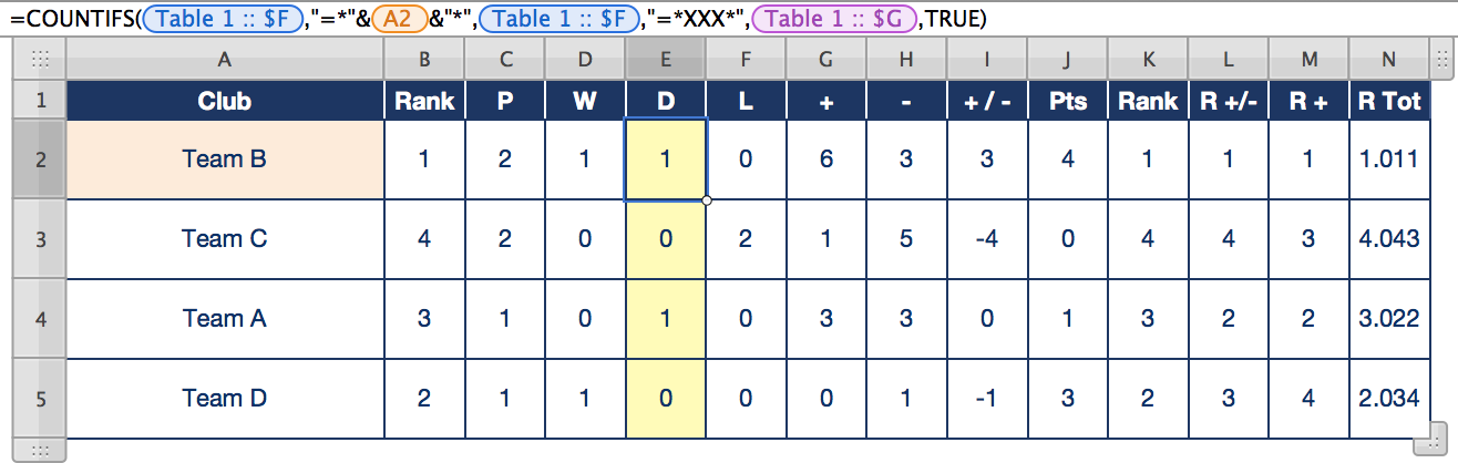
The formula below is entered in D2, and filled down to D5:

D2: =COUNTIFS(Table 1 :: $F,"=*"&A2&"*",Table 1 :: $F,"=*XXX*",Table 1 :: $G,TRUE)

Syntax for COUNTIFS is COUNTIFS(test-values,condition,test-values,condition,test-values,condition)

There are two tests on values in column F:

• Does it contain the team name for whom we are counting draws?
• Does it contain the string "XXX" (Has the game been played?)

There is one test of the values in column G:

Is the value TRUE? (Do both teams have the same score—including both having no score–?)

If all three conditions are TRUE, the row (game) is added to this teams Draw count.

Regards,

Barry

Message was edited by: Barry (Deleted original formula from T 1-1::D2, which I had stored here.)

Hello

I'd introduce an auxially column F in Table 1 to hold a 4-state flag to represent the relation of scores x, y in the row, i.e.,

blank for x and y are blank

-1 for x < y

0 for x = y

1 for x > y

and use this flag to calculate the W, D, and L in Table 1-1 by using formulae as listed below. I'd also use SUMIFS() in calculating + and - in Table 1-1 for better maintainablitily. Formulae for rows 3 through end are to be generated by filling down the forumlae in row 2.

Table 1

F2    =IF(LEN(C2&D2)=0, "", IF(C2=D2, 0, IF(C2>D2, 1, IF(C2<D2, -1))))

Table 1-1

D1    W
D2    =COUNTIFS(Table 1 :: B, A2, Table 1 :: F, 1)+COUNTIFS(Table 1 :: E, A2, Table 1 :: F, -1)
E1    D
E2    =COUNTIFS(Table 1 :: B, A2, Table 1 :: F, 0)+COUNTIFS(Table 1 :: E, A2, Table 1 :: F, 0)
F1    L
F2    =COUNTIFS(Table 1 :: B, A2, Table 1 :: F, -1)+COUNTIFS(Table 1 :: E, A2, Table 1 :: F, 1)
G1    +
G2    =SUMIFS(Table 1 :: C, Table 1 :: B, A2)+SUMIFS(Table 1 :: D, Table 1 :: E, A2)
H1    -
H2    =SUMIFS(Table 1 :: D, Table 1 :: B, A2)+SUMIFS(Table 1 :: C, Table 1 :: E, A2)

Hope this may help,

H

@ Hiroto,

"Hope this may help,"

I like it. Much cleaner with a single column and a four state flag, and with a consistent approach to the two sets of 'totals' formulas (W, D, L and +, - ).

Regards,

Barry

🙂

Embarrassed to see silly typos in my post.

auxially => auxiliary

maintainablitily => maintainability

Hands shivered...

Regards,

Hiroto