using function to calculate values of strings

HI Aymanala,

You wrote: "I need to calculate the total price of "Wifi" and "Model" together as much as they will be repeated"

In the portion of the table you show, the total will be zero. Neither "Wifi" nor "Model" occurs at all in column B. Perhaps you mean "Wi-fi" and "Modem", each of which occurs twice.

What do you mean by "together"?

For the example shown, would the "total price" be $37.60, or some other value?

Could you clarify the problem statement, please.

Regards,

Barry

The function you need is SUMIF then.

In the cell where you want to calculate this, enter the formula below. The formula assumes the name of the table shown in your initial post is "Data", that row 1 is a Header row, and that the formula will be placed in cell C2 of a separate table, and that the text "Wi-fi" is in cell A2 of that table.

For the example, I've used "WF" for "Wi-fi" to cut out some typing.

=SUMIF(Data::$B,A2,Data::$C)

Syntax for SUMIF is: SUMIF(test-values,condition,sum-values)

In the formula:

-- the test values are in column B of the table named "Data"

-- the condition is that those test values must be (equal to) the value in B2 (of the table containing the formula)

-- the sum-values are in column C of the table named "Data"

Sum values on rows where test values meet the condition will be included in the sum.

Using a cell reference to specify the condition permits filling the formula down the column to calculate totals for other values. Numbers adjusts the formula to refer to the column A cell on the new row, and all that's needed from the user is to enter the name of that item to the cell, taking care to exactly match the spelling of the item in the Data table.

Regards,

Barry

$ is the absolute reference operator. B is a reference to 'all the non-header cells in column B, $B fixes that reference to the same cells when the cell's contents are filled to other cells (or placed in other cells using Copy/Paste). In this case, the $ is probably not necessary, as we are not filling the formula into other columns.

A2 is a reference to cell A2. $A2 makes the column reference 'absolute,' fixing it on column A, but leaves the row reference 'relative'. A$2 leaves a relative reference for the column, while making the row reference 'absolute'. $A$2 makes both the column and row reference absolute (fixed).

In th formula, the reference in the formulla in B2 is A2. As the formula is filled down the column, that reference changes—in B3, it will be to A3, in B4 to A4—alway to the cell in the same position—one cell to the left in the same row—relative to the cell now containing a copy of the formula.

For more than one condition, what you'd do depends on how the conditions apply.

Do you want to include the amounts where 'this' is true OR 'that' is true, and exclude the amounts where neither of these is true? If so, use two SUMIF statements and add the results.

Or do you want to include only those amounts where 'this' is true AND 'that' is true? If so, then use SUMIFS.

Here's an example, using my earlier tables, with added data:

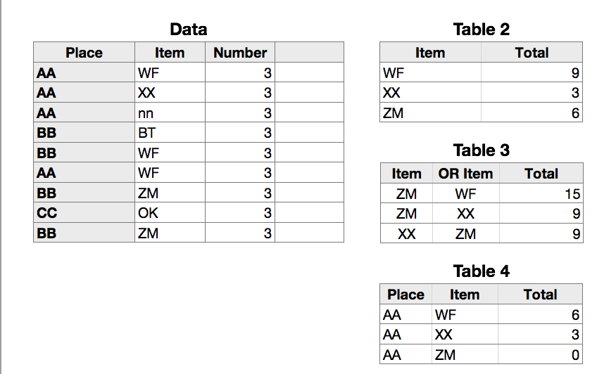
Table 2::C2 has the same formula as before: =SUMIF(Data::$B,A2,Data::$C)

Table 3::C2, and filed down: =SUMIF(Data::$B,A2,Data::$C)+SUMIF(Data::$B,B2,Data::$C)

Each of the conditions (=ZM and =WF in row 2) is evaluated separately. If either is true, the amount is included in the total.

Table 4::C2: =SUMIFS(Data::$C,Data::$A,A2,Data::$B,B2)

Both conditions (Place =AA and Item =WF in row 2) must be true for the amount to be included in the total.

Regards,

Barry