Numbers for simple school data

To get you started.... in addition to looking (via your menu) at Help > Numbers help to get a general feel for how things work, you should have a look at Grade Book and GPA under Education templates (File > New and look in the template chooser):

SG

Hi Kipp,

Welcome to the Numbers Discussions. I gather that you were intending to post a screen shot to show us your data, but if so it didn't make it. Shift-Command-4 to activate the screen grab selection tool, and after you've made the capture, click on the camera icon and follow the instrucitons in the dialog box. Your screen shot graphic will be on your Desktop.

Sounds like you want to keep it simple for this first episode with spreadsheets, so that's what we will try to do for you.

Jerry

Kipp,

I still do not see enough context to undestand what is compared to what. (GCSE) and Media Mock Grade do not mean anything to me. Perhaps you can describe a little more what you want to do.

KippMajors78 wrote:

I did indeed - sorry. VERY new I should ADD!

OK, got some data. Now what would you like the outcome to look like?

Jerry

Is something like this what you are looking for?

SG

Ok, here are some ideas.

The Data table is just data, no formulas.

The Count table counts the occurrences of each grade.

You list the possible grades in column A.

Then in B2, you try a formula like this:

=COUNTIF(Data::A,$A2)

In the formula editor it will look like this:

If it gives you the result you expect, then copy it down and right in that table.

Add a Footer Row at the bottom.

In the cells there put =SUM(B) and =SUM(C)

Then set up a Percentage table:

The formula in B2 there would be

=Count::B2÷Count::B$9

Copy that to the other body cells in that table.

Make sure the shaded rows are defined as Header row.

SG

then getting a percentage for say the 1st 2 rows (A-B), then 1st, 2md 3rd rows (A-C)

A simple way to do this might look like this:

I just set up an additional 'Count Consol' table, and put in the formula in cell B2:

=SUM(Count::B2:B3)

Then copied it to B3.

And in C3 I put

=SUM(Count::B2:B4)

Then copied it to C3.

And in the 'Percentage Consol' table I put in B2:

=Count Consol::B2÷Count::B$9

And copied it right and down.

I don't type all that in. Type = and the formula editor appears, enter the function and where you need a range of cells you can select the range with your mouse (or trackpad) and Numbers will enter the range for you, including the table name.

This is just one way to do this. There are other more elegant ways. But it should give you an idea of how you can approach the problem in Numbers.

SG

Hi Kipp,

You wrote:

- percentages of A-Bs and A-Cs etc per the two classes

For this, you'll need to count the number of each letter grade, then divide the sum of the counts for grades in the range you want to compare by the sum of the counts for all of the grades. The result will be a decimal fraction. Format the cell to display as percentage. In the example below, these results are shown in Table 2.

- if possible, highlight where my subject was higher/lower than the other results for that student (I've removed the names column for purpose of showing my data)

This can be done using conditional formatting to compare the cell containing your student's grade with the cell containing the other teacher's grade for the same student. Done most conveniently if you have the grades in adjacent columns. In the example below, this is shown on Table 1.

Example:

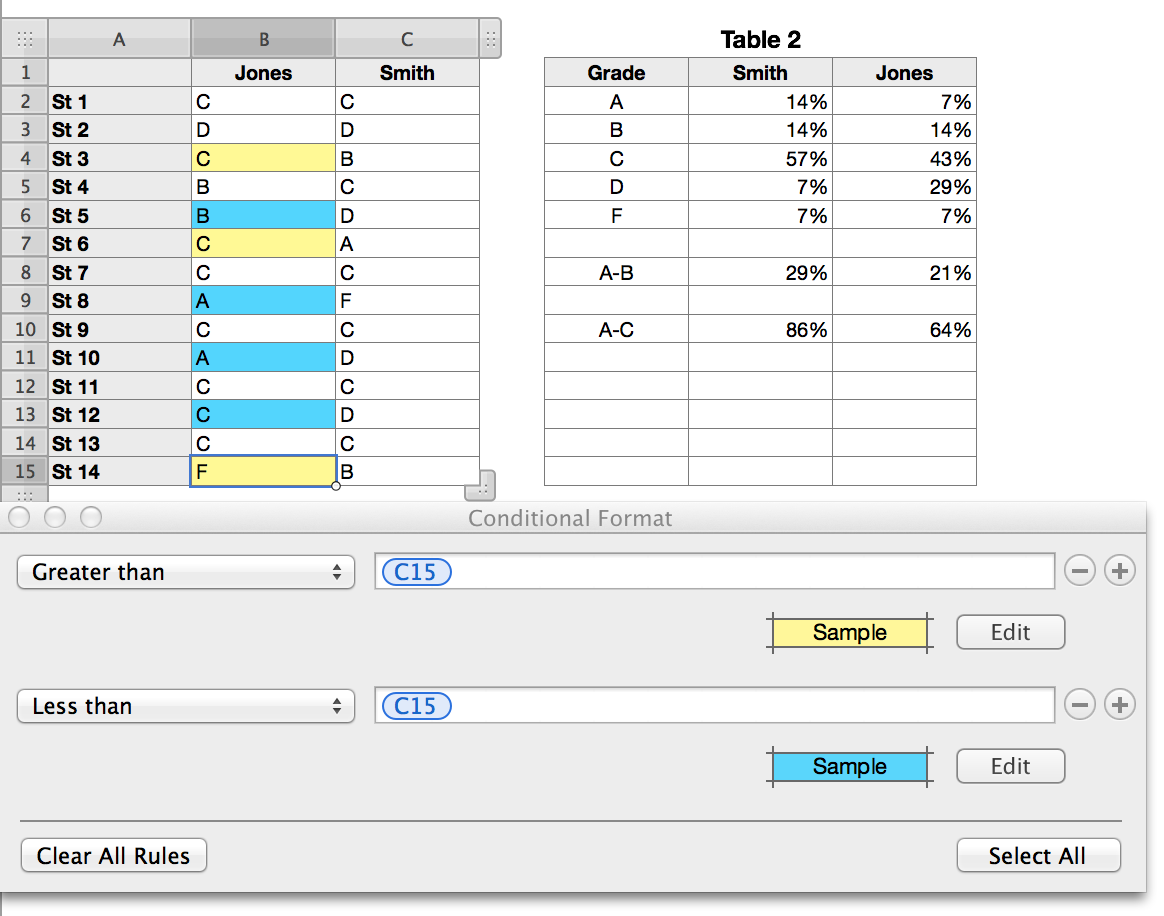
Table 1 (Left):

All data shown has been randomly generated for the example. In your case, this data would be pasted in from your grade book and from your colleague's.

The conditional format rules for cells in column B are shown for cell B15 (selected). The other rule sets are the same, but the two cell references shown are made to the cell in the same row of column C as the row of the cell to be formatted. See Numbers Help for details on how to do this.

Table 2:

There are three versions of essentially the same formula here.

B2, filled right then down to C6: =COUNTIF(Table 1 :: B,$A2)/COUNTA(Table 1 :: B)

B8, filled right to C8:

=(COUNTIF(Table 1 :: B,$A2)+COUNTIF(Table 1 :: B,$A3))/COUNTA(Table 1 :: B)

B10, filled right to C10:

=(COUNTIF(Table 1 :: B,$A2)+COUNTIF(Table 1 :: B,$A3)+COUNTIF(Table 1 :: B,$A4))/COUNTA(Table 1 :: B)

Each instance of COUNTIF counts the items in column B of Table 1 that match the grade listed in the specified cell of Table 2.

COUNTA counts all on the text entries in column B of Table 1.

Example is constructed in Numbers '09. Appearance will differ slightly in Numbers 3.

Regards,

Barry

Kipp,

You may find that graphical comparisons are helpful. Here are some examples for the set of grades on the right of your post...

Jerry

KippMajors78 wrote:

Thanks Sg - looks brillaint. But some reason I can't get 'data' in my formula editor. What am i doing worng?

The Data is the name of the table I have in my example. Numbers will fill it in the table name for you if you click on that column. You enter a table name by checking 'Table Name' in the Table inspector at right, then editing the name above the table.

SG