Looks like no one’s replied in a while. To start the conversation again, simply ask a new question.

EXCEL INDIRECT not supported in NUMBERS?

Although this refers to NUMBERS on an iPad, it was suggested I try this forum as more users here may have run into this situation on the Macs. I imported an EXCEL spreadsheet into NUMBERS on an iPad, but any formula containing an INDIRECT function was removed leaving only the last value available. Is there some incompatibility for INDIRECT between EXCEL and NUMBERS? Is there any workaround to get by this?


Thanks,


JohnD

Posted on Jul 5, 2014 1:48 AM

Reply
13 replies

Jul 5, 2014 7:15 PM in response to SGIII

I have created a spreadsheet that calculates the position of alignment stars for a telescope. There are four sheets within the workbook. Some sheets access data from other sheets. The INDIRECT function is absolutely essential for this to work. Here is an example of one cell:


=IF(INDIRECT("$A$"&ROW())<>"",INDIRECT("Align_Stars!$A$"&INDIRECT("$A$"&ROW())) ,"")


This particular cell extracts data from another sheet based on a value in the first cell (column A) of the current row. The cell in the first column indicates what row in the other sheet from which the data will be extracted. I played with some test statements in NUMBERS and it looks like there is a distinct difference in how EXCEL handles the INDIRECT statement and how NUMBERS handles it which might explain why NUMBERS removes formulas containing INDIRECT. Below are some screen prints.


JohnD


User uploaded file


User uploaded file

Jul 6, 2014 5:54 AM in response to SGIII

It was a bear to put together but it works nicely in EXCEL. I did not give you a good image of the "Available" sheet. Here is a better one showing you the rows and columns. The formula is in cell C9. It tests to see if something is populated in column "A" first before extracting the star name from the "Align_Stars" sheet.


JohnD


User uploaded file

Jul 6, 2014 8:05 AM in response to johnpdap

It seems that each row on your Part 3 extracts values from selected columns from Part 2 for that star.


One way you could do that would be something like this:


User uploaded file


The formula in B2, copied right and down, is:


=INDEX(Align_Stars::$A:$L,MATCH($A2,Align_Stars::$A,0),MATCH(B$1,Align_Stars::$ 1:$1,0))


This retrieves the value in the Align_Stars table where the star name and value in the column header match.


Your table probably goes beyond column L. In that case change L to your last column. To do that I generally click the address token (the blue one here) and select all the columns in the table.


The spelling (but not the case) needs to match in the two tables.


Then, you can add columns to the right for your x's.


Note that in Numbers it's generally more efficient to have compact tables with a Header Row and body cells, as opposed to Excel where you often have expanses of empty cells.


SG

Jul 6, 2014 8:03 PM in response to johnpdap

Numbers has the INDIRECT function. Remember that INDIRECT uses a string value that represents the cell address. Excel and Numbers address cells differently when the cell is on a different worksheet/table. Excel uses an exclamation point ( Worksheet!cell ) while Numbers uses a double colon ( Sheet::Table::Cell ). Strings do not get modified during import/export so the string being used in the INDIRECT function stays the way you wrote it. It will fail in the other app.


I think you could use IFERROR to solve it:


=IFERROR(INDIRECT(Excel's addressing method), INDIRECT(Number's addressing method))

Jul 7, 2014 3:05 AM in response to SGIII

Hi SGIII,


Let me explain a little further as to what is going on. If you look in the Align_Stars sheet (which is the "Part 2: Alignment Stars List"), you will see column "L" labeled "Vis". You see a mixture of blanks and "Y"'s. That column represents any star within a certain altitude range. These are the stars I want. The "Available" sheet looks for those lines in the Alignment Stars sheet with the "Y" in the "Vis" column and populates the "Available" sheet with them. I use a MATCH statement for that:


=IF(INDIRECT("$A$"&ROW()-1)<Align_Stars!$D$6, MATCH("Y",INDIRECT("Align_Stars!$L$"&INDIRECT("$A$"&ROW()-1)+1&":"&"$L$"&INDIRE CT("Align_Stars!$D$6")),0)+INDIRECT("$A$"&ROW()-1),"")


This statement picks up the row number of a line that contains the "Y" which then allows me to populate all the relevant data from "Align_Stars" sheet. The problem is that I need to start the next line's MATCH one row after the previous match. This is can do by adding 1 to the row number of the previous match [INDIRECT("$A$"&ROW()-1)+1]. Since it will give me a row number relative to where I started the MATCH, I also need to bump the result by the row of the previous MATCH (+INDIRECT("$A$"&ROW()-1). It works very well in EXCEL. This is the key to building the "Available" sheet. I have been playing with the ADDRESS function to replace the INDIRECT's but have been unable to get that to work.


JohnD

Jul 7, 2014 4:32 AM in response to johnpdap

Ah, yes, the function is removed during import. Probably no workaround for it then.

The problem is not the import of sheet references. INDIRECT does not contain any sheet or cell references, it contains a string and turns that string into a reference. the strings used for Excel are different than those used for Numbers if they reference cells outside of the current table. It would be very difficult if not impossible for import to modify the strings except in the most easy case where the string is all contained in quotes, not created from a formula.

Jul 7, 2014 7:54 AM in response to johnpdap

You could rewrite your formula using OFFSET or INDEX instead of INDIRECT. Those functions use actual cell references, not strings, and they should get converted during import/export.


I did not test this but here is what I am thinking:


=IF(OFFSET($A$1,ROW()-1,0)<>"",OFFSET(Align_Stars::$A$1, OFFSET($A$1,ROW()-1,0),0) ,"")

Jul 7, 2014 1:22 PM in response to johnpdap

The "Available" sheet looks for those lines in the Alignment Stars sheet with the "Y" in the "Vis" column and populates the "Available" sheet with them.


Here's a "Numbersy" way to do that. Add an "index" or "counter" column to your Align_Stars table that you can hide later if you want. I've called mine VisCntr.


User uploaded file


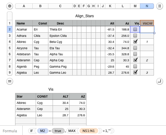
The formula in N2, copied down is:


=IF(M2=TRUE,MAX(N$1:N1)+1,"")


All this does is increment a counter whenever it finds a TRUE value (a checked checkbox) in the 'Vis' column.


Then, in column A2 of the other table (I've called the table 'Vis') place a formula that looks like this, and copy it right and down:


User uploaded file

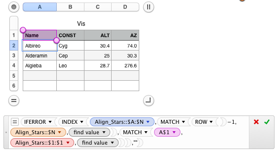
=IFERROR(INDEX(Align_Stars::$A:$N,MATCH(ROW()−1,Align_Stars::$N,0),MATCH(A$1,Al ign_Stars::$1:$1,0)),"")


In row 2, the formula subtracts 1 from its current row 2 to get 1, and looks up the 1 in the 'VisCntr' column. When it finds it, it returns the value in matching column of 'Align_Stars'... And so on for the following rows. The IFERROR is simply cosmetic, to suppress red warning triangles.


An advantage of this approach is that you can easily insert additional columns into your 'Vis' table, give them headers whose spelling matches what you have in 'Align_Stars', and just copy the formula over into the new columns to populate them with the correct values.


I find this approach easier and more flexible than struggling with INDIRECT and OFFSET.


SG

Jul 8, 2014 3:13 PM in response to SGIII

I am in the process of redoing the spreadsheet, trying to eliminate as many INDIRECT's as possible. If I can cut them down to a manageable number where I just need to re-enter formulas in a few columns, that might work. I found that EXCEL has a problem accessing an array referencing another sheet when the reference is isolated in a cell. NUMBERS is ok with that. With EXCEL, if you build the reference "in-line" in the formula, it works. I will also try some of your suggestions to see if they work. I will check back in a day or so.


JohnD

Jul 10, 2014 11:56 PM in response to johnpdap

SUCCESS. I was able to finally transfer over the EXCEL file to the iPad and with a minimum of changes on the NUMBERS side and get it to work. There were two columns and a handful of single cells which contained INDIRECT statements and required re-entering on the NUMBERS side. Now that I have it working there, I can do some fine-tuning on the NUMBERS side if necessary. Working on the IPad mini can be difficult when you are dealing with small cells. There are times when I try to select a cell and it refuses to take it especially if that cell is already part of the formula. I was able to copy that entry in the formula however, so I could get it to work. Tapping the correct cell can sometimes be challenging as well. I need to get a "fine" stylus to work on something like this.


Thanks for all your help,


JohnD

EXCEL INDIRECT not supported in NUMBERS?

Welcome to Apple Support Community
A forum where Apple customers help each other with their products. Get started with your Apple ID.