Hi Grand'
"(T)his is just a numbering system, not for any additional info other than to classify a photo according to its given number."
"11.10 is a different photo from 11.100. I would like 11.99 to be followed by 11.100."
Your described use implies that part of the number identifies a "class" or group to which a particular photo belongs. My assumption is that the first part of the number identifies this "class" (eg. nature, action, architecture, etc. or photographer, or camera). The second part appears to be a serial number assigned to each photo in this class.
You want a sort that sorts all of the photos by their category (the number to the left of the dot), then sorts within each category by the serial number part (the number to the right of the dot). There are two ways to go about this:
- Separate the category and the serial number into two columns, then do a double sort, first by the serial numbers, then by the categories.
- Rewrite the existing ID into a sortable form.
Hiroto's "sorting key" column (in column B of his table) takes the second approach.
The first part of his formula— VALUE(LEFT(A2,FIND(".",A2)-1))*1000000— pulls out the characters to the left of the ".", interprets them as a number, then multiplies that number by 1000000 to ensure that none of the original digits will be changed by adding the result of the second part.
The second part—VALUE(RIGHT(A2,LEN(A2)-FIND(".",A2)))— pulls out the digits to the right of the "." and interprets them as a number.
The two numbers are then added to produce a single number. That number will always start with the digits that are to the left of the "." in the original ID. Those digits will always be followed by six more, ending with the digits that were to the right of the "." in the original ID.
The full number will sort in the order you are looking for.
(The random numbers in Hiroto's column C provide a means of re-sorting the table into a random order. As Hiroto states, that column is there for testing purposes; It would not be included in your table.)
The approach I numbered "1" uses a pair of formulas, each essentially the same as part of Hiroto's method:
C2 and filled down: =VALUE(LEFT(B,FIND(".",B)-1))
D2 and filled down: =VALUE(RIGHT(B,LEN(B)-FIND(".",B)))
Sorting the table, first on column D, then on column C, gives the results shown below:
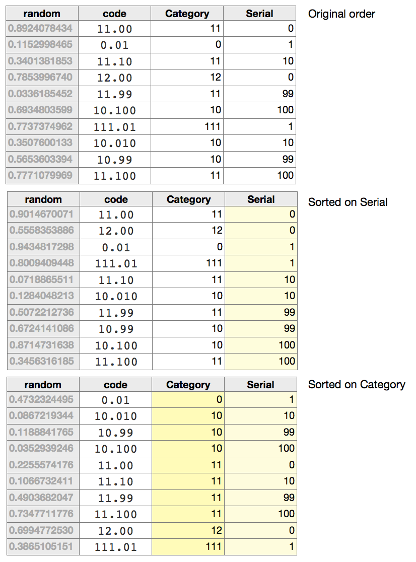
Note that the text values "11.00" and "12.00" in column B drop the second zero when converted to numbers in column D. As your example shows no values that end ".00", I've assumed these do not occur in your list, and the dropped digit will cause no problems.
"I also tried the Custom, but that didn't work either. I didn't know how to "Add a Rule.""
"Add a rule" in the instance displayed will either allow you how to display "special" values such as zero or numbers less than zero, or will permit you to add conditional formatting rules that compare the value in the cell with another value and apply colour fill or colour text depending on the result of the comparison. Unlikely to be of any help in the issue under discussion.
Regards,
Barry