Numbers automatic fill new spreadsheet list and Sum

Hi BizzBro,

SUMIF is your friend.

Formula in List 2 B2 (and Fill Down)

=SUMIF(List 1::A,A2,List 1::B)

Regards,

Ian.

Hi BizzBro,

You want to find unique values in table List 1 and populate List 2 with them.

I thought SG had an apple script to do this. Maybe he will stop by and show us a script where we don't need all these extra columns and formulas.

You get SUMIF so I will focus on populating column A of List 2.

We will need additional columns.

List 1 on the left.

B2 =IF(COUNTIF(A$2:A2,A2)=1,A2,"")

C2 = 2

C3 =IF(LEN(B3)>0,MAX(C$2:C2)+1,"")

For the payoff, List 2

A2 =INDEX(List 1::A,MATCH(ROW(cell),List 1::C,0))

I would make List 2 plenty long and hide extra rows with a filter.

quinn

Hi Bizzbro,

Me too.

quinn

HI Quinn & BizBro

Column B of "List 1" is unnecessary. Here's a variation that eliminates that column (and the calculations it makes).

List 1::B2: =IF(COUNTIF($A$2:A2,A)=1,MAX($B$1:B1)+1,"")

Fill down

List 2::A2: =INDEX(List 1::A,MATCH(ROW()-1,List 1::B,0))

Fill down

List 2-1 is a duplicate of List 2, using the same base formula, but placing it in an IF statement that suppresses calculations (thus avoiding the error message) after the maximum index value has been reached. Added parts in bold below.

List 2-1::A2: =IF(ROW()-1>MAX(List 1 :: B),"",INDEX(List 1::A,MATCH(ROW()-1,List 1::B,0)))

Regards,

Barry

Hi BizzBro,

VLOOKUP() would do it for you as long as your search term is in a column before the return column. I have been using the combination INDEX/MATCH because it has so much flexibility.

The second table would be your list 2. Match finds the row and index determines the column.

quinn

HI BB,

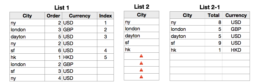
The only use made of IF in Quinn's solution, or in mine, is to create the index column used to determine which rows will provide the list of city names for List 2. INDEX, or one of the LOOKUP functions is used to transfer the data to List 2.

IF can be used (as it is in List 2 - 1 below) to determine if there is a need to transfer data in each row.

Formulas

List 1:

Columns A, B and C contain entered data.

D2: =IF(COUNTIF($A$2:A2,A)=1,MAX($D$1:D1)+1,"")

This is the same formula as used in my earlier post. The range for MAX is now in column D to match the new position of the index column. I prefer to have these in the last column of the table (and hidden) to get them out of the 'danger zone' where data is being entered.

IF is used here to tell the formula to add 1 to the MAX value only on the row where a city name first appears.

List 2-1

A2: =IF(ROW()-1>MAX(List 1 :: $D),"",INDEX(List 1::A,MATCH(ROW()-1,List 1::$D,0)))

Same formula as in previous example, with the index reference changed to column D to match the new location, and made absolute ($) to keep it there as the formula is filled or copied into column C.

The formula in A2 was filled right to B2 (temporarily) and C2

C2: =IF(ROW()-1>MAX(List 1 :: $D),"",INDEX(List 1::C,MATCH(ROW()-1,List 1::$D,0)))

The only change from the version in column A is the part shown in bold, which tells Numbers to get the (currency) values from column C of List 1.

B2: The filled right formula from column A would retrieve only the first order value from each city. As we want the total, it must be changes to a SUMIF formula.

As in the other formulas, the working core will be enclosed in an IF statement to suppress calculations where they are not needed. The test is for an entry in the City column.

B2: =IF(LEN(A)>0,SUMIF(List 1 :: A,A2,List 1 :: B),"")

Select cells A2, B2 and C2 on List 2-1, and Fill down to the end of the columns.

Regards,

Barry