Highlighting a cell based on true/false value of another cell

Hi rjc,

Conditional highlighting rules depend on comparing the value contained in the cell to be highlighted (D2) with a second value. The second value may be fixed (recorded in the rule) or may be contained in a second cell.

In your described scenario, the highlighting would be independent of the value in D2.

There are two ways to accomplish what you want using conditional highlighting—by highlighting a third cell whose value is dependent on the value in H2, and whose highlighting will be perceived as highlighting of D2, OR by providing a third cell whose value can match or not match the value in D2, depending on the value in H2.

Since you want to highlight only a single cell, and not a group of cells, the second method is probably simpler here.

Each cell in clumn I contains the formula below, entered in I2, then filled down through the rest of the column:

I2: =IF(H,D,"xxx")

English: If the cell in this row of column H is TRUE (checked), copy the value in this row of column D to this cell. Otherwise, put "xxx" in this cell.

"xxx" may be any value that will never be present in the cells of column D.

The conditional format rule shown below the table is placed in cells D2 - D10. The cell reference is for the cell on 'this row' in column I, and is different for each cell.

Regards,

Barry

The 'other' method, useful if you want to highlight more than a single cell in each checked row, is shown here.

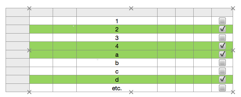
WHat was the added column, I in the example above, is now a single column table, sized to exactly underlay columns B through H of the first table when slid behind that table. In the image, this new table has been selected and locked. The x s show the location of the corners and centres of each edge.

The formula in column A of the new table is the same as that in column I above, edited by Numbers to add Table 1 to the cell references as it is now referencing cells in columns D and H of a table not containing the formula.

A2: =IF(Table 1::H,Table 1::D,"xxx")

Filled down as described above.

All rows of Table 2 (the new table) have been set to Fill White and Text White as the normal setting.

These cells have also been given a conditional format setting to set the fill and text to the green shade shown when the condition is met.

The condition, " 'Equal to' Table 1::D2" in the case of cell Table 2::A2, compares the same cells as the example above, but the rule is now in, and works on, the cell containing the formula, not the one with the original data.

Body cells in Table 1 have been set to have no fill, as has Table 1 itself, making all cells in the body of that table transparent, allowing the formatting to be seen on the table behind.

Regards,

Barry

"Stupid question here, but how do you open the Conditional Format window?"

Hi rjc,

The only 'stupid questions' are the ones that don't get asked.

In Numbers 3, Conditional Formatting is called Conditional Highlighting. Even with the name change, it's found in the Format section.

Select one or more cells.

Click on the Format brush, then on Cell, then on Conditional Highlighting, then on Add a rule.

Further details available in the Knowledge Bank article here.

Regards,

Barry