Looks like no one’s replied in a while. To start the conversation again, simply ask a new question.

Conditional Formatting In Numbers

I have conditional formatting set up on a cell, its a due date so it is yellow just before, then orange and red for overdue.


There is another column that has the name of an individual, I need to mirror the colour of the conditional formatting to this cell but it will obviously have text in it. Is this possible? If so what formula would I use for this?

iMac, OS X Yosemite (10.10.5)

Posted on Apr 14, 2016 3:53 AM

Reply
Question marked as Best reply

Posted on Apr 14, 2016 6:56 AM

Hi pobiom,


This is the same question you asked here: Conditional Formatting.

In that answer the data column would hold the name of the individual. It specifically answers this question.


If you don't understand something I will try to explain it to you.


quinn

7 replies

Apr 27, 2016 3:41 AM in response to pobiom

Hi Quinn,


Sorry for the delay in getting back to you. Would you mind explaining this one again if possible, I am not very technical. Attached is the example of what I have so far.


User uploaded file


The date is a due date and the closer to the date the cell will change colour, what we would like to happen is for the cell next to match the colour of the conditional formatting of the date cell.


Many thanks for your help, it is appreciated.


Best regards

Pobiom

Apr 27, 2016 7:21 AM in response to pobiom

Hi pobiom,


As you can see in this thread Conditional Formatting, Numbers does not have a way to adopt the formatting of one cell to another. In order to highlight your cell there we needed to create an extra column and recreate the formatting when your conditons are met.


It is looking like you are now proposing three different conditions for three different highlights. This can be done by repeating the solution offered above. You will end up with three aditonal columns. Have you attempted to make that solution work? Start with your simplest case. In my example the highlight was triggered when the date passed. the formula in the extra column was:

User uploaded file

If the date in A2 was less than (earlier) today then the cell would match the value in B2. If B2 and C2 matched then the highlight is applied.


So design your formulas to reflect the cases you want to test for.

IF(A5−7<TODAY(),B5,"") will match if A5 is within 7 days of today.


Try these out and ask spefific questions about waht you cannot get to work.


quinn

Apr 28, 2016 12:02 PM in response to pobiom

Three conditional highlighting rules can be accommodated with a single auxiliary column, as shown below. (The small table, showing today, is included only to show the current date when the screen shot was taken, and is not used in the solution.

User uploaded file

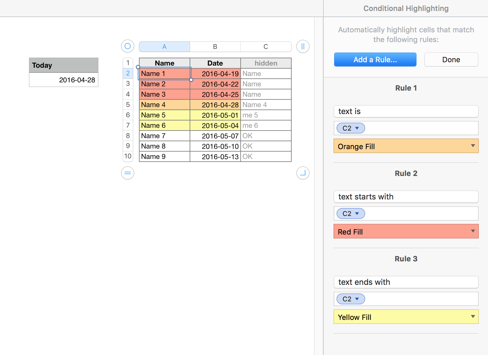
Column C contains this formula:

C2: IF(B<TODAY(),LEFT(A,4),IF(B=TODAY(),A,IF(B<TODAY()+7,RIGHT(A,4),"OK")))

Fill down to the end of column C.


Note: I had originally used a null string ( "" ) where "OK" is used in the formula, but found that this would fill the "text starts with" condition and place a red fill in the cell for any 'name' in A. "OK" works for the example, but would produce erroneous results for a name such as "Oklahoma Jones" or "Tim Cook".

A longer string, using a single repeated character, such as "zzzzzzz" would likely avoid the possibility of false matches to the CH rules shown.


Conditional highlighting rules for the Date column are shown here:

User uploaded file

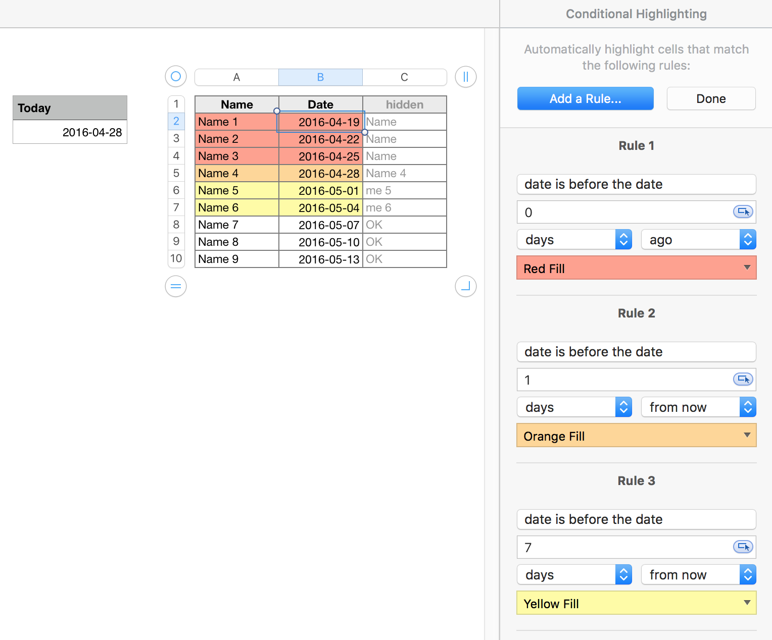
Order of the rules is important. Numbers evaluates the rules one at a time, starting at Rule 1, applies the highlighting whose condition is first met, and does not look at any later rules in the list.


Regards,

Barry

Conditional Formatting In Numbers

Welcome to Apple Support Community
A forum where Apple customers help each other with their products. Get started with your Apple ID.