Sorting/Replacing by Internal Character

you can do this without sorting by following this example:

In column A is the original names

B1=IFERROR(FIND("(", A1), 0)

this is shorthand for... select cell B1 ,then type (or copy and paste from here) the formula:

=IFERROR(FIND("(", A1), 0)

C1=IFERROR(FIND(")", A1,start-pos), 0)

D1=IF(AND(B1>0, C1>0), LEFT(A1, B1−1)&RIGHT(A1,LEN(A1)−C1), A1)

select cells B1 thru D1, copy

select cells B1 thru the end of column D, paste

now column D contains the "corrected" names. select column D copy

now select the destination and use the menu item "Edit > Paste Formula Results"

David Blomstrom wrote:

1) sort columns according to special characters the various values contain, and 2) delete all parentheses and everything they contain

Taking 2) first, here is one way, using a single formula:

In cell B2, filled down:

=IFERROR(SUBSTITUTE($A2,MID($A2,FIND("(",$A2,1),FIND(")",$A2,1)−FIND("(",$A2,1) +2),""),$A2)

For 1) to mark the entries that originally included ( ) for sorting if you want, the formula in C2, filled down:

=A2<>B2

SG

Hi David,

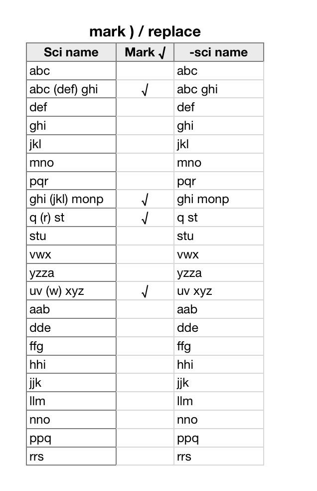
You can't sort on "contains (", but you can filter the table on that column with the rule 'text' 'contains' '(' to show only the rows containing parentheses, then mark all the visible rows with a √ in your added column.

OR you can do the marking automatically, using the formula in the added column (B).

AND you can do the removal automatically using the formula in column C. (see notes below)

Formulas (entered in row 2 and filled down to the end of the column):

B2: =IF(ISERROR(FIND(")",A,start-pos)),"","√")

Find returns a number if the closing parentesis ( ")" ) is found, and an error is it is not.

ISERROR returns TRUE if there is an error, FALSE if there is not.

IF returns a null string ( "" ) on TRUE, a check mark ( "√" ) on FALSE. You can get a better checkmark from the character viewer—Show emojis and symbols in the input menu, which displays as a flag indicating the keyboard layout you are using.

C2: =IFERROR(REPLACE(A,FIND(" (",A),FIND(")",A)+1−FIND(" (",A),""),A)

FIND(" (",A) returns the position of the space before the opening parenthesis (4 in A3), used by REPLACE as the position to start when replacing the string.

FIND(")",A)+1 returns one more than the position of the closing parenthesis (10 in A3), and

-FIND(" (",A) repeats the first find, and subtracts the result (4) from the result of the second find (10-4); REPLACE uses the result to tell how many characters to replace.

"" tells REPLACE what (a null string) to insert as the replacement for the selected characters.

The first FIND will throw an error if it cannot find " (" in the string in A. That is caught by IFERROR, which skips the rest of the calculation and goes to the last argument, ( A) which tells it to place the contents of the cell in this row of A into the cell containing the formula.

CAUTION: Formulas are 'live.' Their results change when the data in cells they reference changes. To preserve the values in columns B and C you must, before editing column A:

Select all of the cells in columns B and C, and Copy.

With the cells still selected, go Edit (menu) > Paste Formula Results.

This replaces the formulas in these columns with the results last calculated.

You may then want to Copy the cells in column C and Paste into column A, then delete column C, leaving the shortened names in A, and the checkmarks in B.

Regards,

Barry

Barry's use of REPLACE is more succinct than SUBSTITUTE.

=IFERROR(REPLACE(A,FIND(" (",A),FIND(")",A)+1−FIND(" (",A),""),A)

vs.

=IFERROR(SUBSTITUTE(A,MID(A,FIND("(",A,1),FIND(")",A,1)−FIND("(",A,1)+2),""),A)

and the explanation (which in essence applies to both formulas in that you're replacing part of the string with "") is great.

SG