create a table as shown on the left of the screenshot (included below so you can copy and paste):
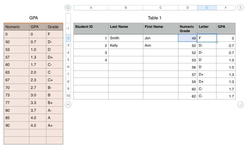
the table should be named "GPA" as shown so the formulas will work:
In the table on the right you can look up the Letter and GPA like this.
enter the numeric grade on column D
select cell E2, then type (or copy and paste from here) the formula:
=VLOOKUP(D2,GPA::A:C, 3,close-match)
short hand for this is
E2=VLOOKUP(D2,GPA::A:C, 3,close-match)
F2=VLOOKUP(D2,GPA::A:C, 2,close-match)
select cells E2 and F2, copy
select cells E2 thru the end of column F, paste
Here is the lookup table information for your convenience:
Numeric | GPA | Grade |
0 | 0 | F |
50 | 0.7 | D- |
53 | 1.0 | D |
57 | 1.3 | D+ |
60 | 1.7 | C- |
63 | 2.0 | C |
67 | 2.3 | C+ |
70 | 2.7 | B- |
73 | 3.0 | B |
77 | 3.3 | B+ |
80 | 3.7 | A- |
85 | 4.0 | A |
90 | 4.0 | A+ |
|
|
|
|
|
|