I need to make tiered values for a cell

Hi Haddy,

Use a lookup table. This makes it easy to edit the thresholds and rates without having to rewrite the formula.

Here's an example, using the rates and thresholds in your post.

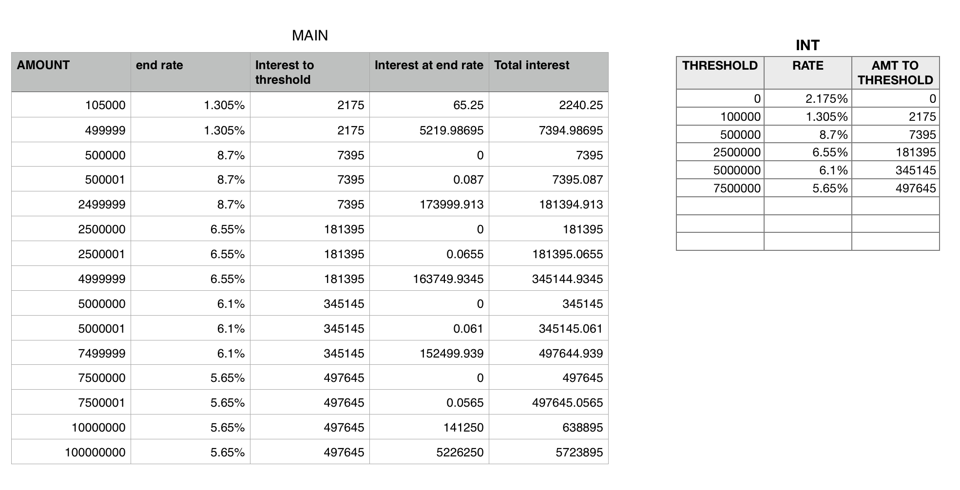
INT is the lookup table.the first two columns are entered data—the threshold amounts in column A, and the interest rate starting at thea threshold in column B.

Column C contains the formula below, which calculates the interest charged up to each threshold.

C2: entered value — 0 (zero)

C3: =(A3−A2)×B2+C2

Fill down to last row requiring this calculation (Row 7 in example).

MAIN is the table on which the interest due is calculated. Amounts are entered in column A, all other values on the table are calculated. Calculation has been spread over four columns to show each step separately. the whole calculation can be done in a single column, using the formula shown below.

All formulas are entered in row 2, then filled down for the number of rows needed for calculating different loan amounts.

B2: =LOOKUP($A,INT::$A,INT::B)

Looks up the interest rate on the amount greater than the last passed threshold amount.

C2: =LOOKUP($A,INT::$A,INT::C)

Looks up the amount of interest charged on a loan at the last passed threshold amount.

D2: =B×(A−LOOKUP($A,INT::$A))

Looks up the last passed threshold amount, subtracts that for the amount of the current loan, and multiplies the result by the interest rate in column B.

E2: =C+D

Calculates the total interest changes by adding the interest due on amounts up to the last threshold and the interest due on the amount above that threshold.

The four formulas may be combined as follows, to return the same result:

F2: =LOOKUP($A,INT::$A,INT::C)+(A−LOOKUP($A,INT::$A))×LOOKUP($A,INT::$A,INT::B)

Regards,

Barry

Another common way to do this allows you to reduce the calculation into a single cell without a lookup table.

The first step is to lay out the tiers similar to the first three rows in this table:

The main idea is to list the lower and upper end of each range.

Then note that the commission (or tax?) in each range can be calculated as follows:

=MAX(0,(MIN(<upper end of range>,<amount>)-<lower end of range>))*<rate for that range>

In the table above this corresponds to this formula in A5:

=MAX(0,(MIN(A$3,$G5)−A$2))*A$1

That formula I copied and pasted into A4:F8 to produce the various examples. G contains the input amounts on which the tiered calculation is applied (since your post refers to G5). H is just a sum of A:F.

Once I made sure the calculations were working correctly I set up row 11 and "hardwired" the upper end of range, lower end of range, and rate in each formula. Normally hardwiring is not good practice but in this case it allows you to combine the table all into one formula that, because of its simple repetition of the pattern, isn't that hard to edit if you change your ranges or rates in the future.

=MAX(0,(MIN(100000,$G5)−0))*0.02175+MAX(0,(MIN(500000,$G5)−100000))*0.01305+MAX( 0,(MIN(2500000,$G5)−500000))*0.087+MAX(0,(MIN(5000000,$G5)−2500000))*0.0655+MAX( 0,(MIN(7500000,$G5)−5000000))*0.061+MAX(0,(MIN(20000000,$G5)−7500000))*0.0565

Note that this looks complicated, but is just the following for each tier you have, added together:

=MAX(0,(MIN(<upper end of range>,<amount>)-<lower end of range>))*<rate for that range>

SG

Six of one, half a dozen of the other, as my mother used to say. 😁

Here's the similar reduction of the Main table in my post above. After inserting that screen shot, I had added another column (F) and entered the combination formula shown for F2: =LOOKUP($A,INT::$A,INT::C)+(A−LOOKUP($A,INT::$A))×LOOKUP($A,INT::$A,INT::B)

At that point the top few rows of the table looked like this:

Reducing the table consisted of selecting and deleting the columns used to perform the interim calculations (B-E),

Then selecting and deleting all the test rows (3-end of the table), and formatting the cells in row 2 to include the thousands separators, and two decimal places in column B.

No changes (except the name) to the lookup table.

Formula in Com::C3 and filled down: C3: =(A3−A2)×B2+C2

All other values in this table are entered data.

Regards,

Barry

Barry wrote:

Six of one, half a dozen of the other, as my mother used to say. 😁

Hi Barry,

I don't presume to "teach my grandmother how to suck eggs," as my mother used to say🙂, but there is a real difference, which is why I posted an alternative to your excellent solution. With the MAX MIN approach you don't have to set up another table, or even a range of other cells in the same table. Everything can be done in a single cell, with the formula surprisingly easy to create and update once you are familiar with its simple pattern.

Then one can display a description of one's tiers "in plain English" as in the original post.

SG

Glad we've got you covered here and that it worked on your end!

SG

Curious...

Hi SG,

I'm getting some strange results with your formula above. Most of these examples agree with mine (as expected), but what's going on in rows 2 and 10?!

Highlighted cell (G2) is empty. G10 contains 100 million.

Formula (copied from the text in your post, then filled up and down from H5 is shown for H2, and repeated in text with the blocks stacked.

Noticed while I was writing that last line, the reason row 10 is lower than I expected—the formula has a cap of 20 million on 'commissionable transactions' in the last block. Reasonable, but not called for in the original discription, which left the top end open.

Still don't see what's going on in H2, though.

Regards,

Barry

Hi Barry,

Perhaps you're putting in values that are so clearly out of range that there isn't much need to error trap in real world use?🙂

No one in my organization would think of trying to get away with calculating on a base of blank! But at the expense of (seldom needed) complexity one could of course test for a blank cell before displaying the result of a calculation.

As for the upper range, it's easy to just change the 20,000,000 to something higher, if one really is dealing up there in the stratosphere way above the next highest range (wish that happened here!).

SG

"Perhaps you're putting in values that are so clearly out of range that there isn't much need to error trap in real world use?"

Perhaps. I was just surprised by it, and wondered what was causing it (and why it matched the result in row 10, which started from a very different input.)

Tried a few variations, dropping off one +MAX(...) section at a time. Results for a blank cell input matched the results for the last maximum value in the last part of the formula remaining.

Of course we don't intentionally calculate on 'a base of blank,' but we also don't expect to see (or get) such a result. Often the results of calculations are passed along and used in a further calculation. With that possibility in mind, it always concerns me to see an abnormal result like that one.

Curiouser and curioser,

Barry

Hi Barry,

If you get any unexpected results in other than a clear edge case such as a blank input cell let us know. This is a common way of approaching the "tiered commission" problem in a spreadsheet.

Probably Conditional Highlighting is the easiest way to alert if the cell is left blank by mistake. Keeps the formula clean.

SG