Still don't get the filtering and the sumif with visible cells

Question

Still don't get the filtering and the sumif with visible cells

Hello all,

I know this is a pain for you people, but i'm really stuck with this problem.

I tried to use the answers i found in the community and User Guide, but I must be closed to this kind of explanation.

So again:

In column A is a serie of dates

In column B the value corresponding

In the B foot row i want the sum of only the visible cells i have filtered previously.

Up to now i always have the sum of all rows, filtered or not.

I added another column with a True/False value and attempted to use it but obtained the same result.

I'm pretty slow at this, so i guess i will need your help once more.

This is the sum before filtering:

And this is the sum after filtering:

Thank you for your time and patience again.

Lionnel

iMac, OS X El Capitan (10.11.3)

Posted on May 1, 2016 11:28 AM

Reply

Answer 1

Best reply

Barry

Level 9

59,861 points

May 2, 2016 3:33 AM in response to lionneldeparis

Hello Lionnel,

Filtering the table affects only which rows are displayed. Hidden rows are still included in calculations by formulas referencing them.

Your formula, =SOMME(B2:B16) sums the contents of all cells from B2 to B16, including any that are hidden.

There are several other functions in the SUM family. SOMME, SOMME.SI and SOMME.SI.ENS are the ones of interest here.

SOMME.SI (English: SUMIF) accepts one condition, and sums only the cells on rows that met that one condition.

SOMME.SI.ENS (English: SUMIFS) accepts several conditions, and sums only the cells on rows meeting all of the conditions.

For the example shown in your post, the formula you need should be:

=SOMME.SI.ENS(B; A; “>=01/02/2016”; A; “<01/03/2016”)

(NOT tested. The dates may need to be placed in two cells, and those cells referenced in the formula. post a reply with any error message if the formula does not work as written.)

The rows not included in the sum do not need to be hidden.

If the formula is placed in column B, it must be in a row defined as a Footer Row using the menu item in the same position as the highlighted one in this screen shot:

Footer rows can be placed only at the foot (bottom) of a table.

Regards,

Barry

Reply

Answer 2

SGIII

Level 8

35,276 points

May 1, 2016 12:17 PM in response to lionneldeparis

Would something like this work for you, where you set up a filter column (that can be hidden)?

The formula in the 'Filtered' column:

=AND(A>=Range::A$2,A<=Range::B$2)

The formula for the filtered sum (cell B18 in the example):

=SUMIFS(B,A,">="&Range::A2,A,"<="&Range::B2)

The filter on column C (to show only the rows between the two dates):

Thereafter you just enter the dates for the range in the second table (I've hidden the Filtered column):

SG

Reply

Answer 3

May 2, 2016 3:33 AM in response to SGIII

Dear SGIII and Barry,

Thans for your reply to my question.

You both gave me the answer I was looking for, that is: use the SUMIFS and find that Filtering is just a visual effect and cannot do the job I was expecting.

Regarding the solution, the SGIII works fine, as the Barry's doesn't. Which is confusing because the Barry's one is more consistent with the SUMIFS protocole described in User Guide.

Indeed, the "&" character is not part of SUMIFS description in my Numbers version. Honestly, I couldn't guess it.

Regarding the visual effect of Filtering, the SGIII solution has the advantage to be simple to use, rather than entering directly with the dates in Filter criteria is longer and subject to typing error. So the TRUE/FALSE column is fine with me.

Here are the pictures of my work:

Maybe you can explain why Barry's solution is not efficient as expected since the idea is the same. What I see is that date references are written in full text rather than appearing as colored

BARRY:

SGIII:

Once again thank you both for your support and time to what appears to be a very common request of Numbers users.

Could Apple take this into account and provide a kind of check box to allow a match between the Filter rule and the calculation rule in one of the cells ?.

Best regards, Lionnel.

Reply

Answer 4

May 2, 2016 4:43 AM in response to Barry

Hello Barry,

Thanks for your reply.

My answer is into this thread with SGIII also, for you both since you found both the solution.

The only glitch in what you suggest is the way it is written: it follows the SUMIFS protocole but doesn't work, as for SGIII it is different from protocole ("&") but it works; and that i wouldn't have found the "&" thing.

The picture of my tests in this thread.

Thank you very much indeed it opened my eyes on something that Filtering cannot do eventually.

Reply

Answer 5

SGIII

Level 8

35,276 points

May 2, 2016 6:58 AM in response to lionneldeparis

Hi Lionnel,

As you probably know, we are just fellow users here. You can give feedback to Apple via Numbers > Provide Numbers Feedback in your menu.

The & is just a concatenation operator that combines strings. From experience I've found when using comparison operators (> < >= <=) with SUMIF, SUMIFS, AVERAGEIF, and AVERAGEIFS that it's a good rule to always wrap the comparison operator in " " and then concatenate it to the rest of the condition using &. Sometimes a formula will work without doing that (as in Apple's selected examples in Formulas & Functions Help) but in many cases it won't. Note that when you are testing for = you can simplify your formula by simply omitting the comparison operator.

Thanks for the feedback and the green tick!

SG

Reply

Answer 6

Barry

Level 9

59,861 points

May 2, 2016 1:41 PM in response to lionneldeparis

"The only glitch in what you suggest is the way it is written: it follows the SUMIFS protocole but doesn't work, as for SGIII it is different from protocole ("&") but it works; and that i wouldn't have found the "&" thing."

Hi Lionnel,

My original form of the SUMIF did 'follow protocole,' but apparently presented the date in a format not recognized as a date within the context of SUMIF.

SG's solution also 'followed protocole,' but, as you've noted, that implementation of the protocol wasn't demonstrated in the examples provided in the function help documents.

The help description of the condition does include 'the "&" thing.' In the English version, it's referred to as "the ampersand concatenation operator," in the French version, "l'opérateur de concaténation esperluette," but again, no examples are provided.

From your screen shot:

Here, because A21 is inside the quotation marks, OS X sees it only as a text string. The & operator is needed to place A21 outside the quotes, where OS X can recognize it as a cell reference and change it to a token. OS X then retrieves the contents of that cell, the operator appends that result to the string inside the quotes, and the resulting text string (as required by SOMME.SIS and other ...IF and ..IFS functions) is read as a condition expression by SOMME.SIS.

English version showing recognition of A21 and A19 as cell reference tokens::

=SOMME.SIS(B2:B16;A2:A16;"<="&A21;A2:A16;">="&A19)

Regarding:

"Could Apple take this into account and provide a kind of check box to allow a match between the Filter rule and the calculation rule in one of the cells ?."

Do Provide Numbers Feedback and make a feature request to Apple. One of the criteria used is the amount of demand for each enhancement, so every request doe add a little weight.

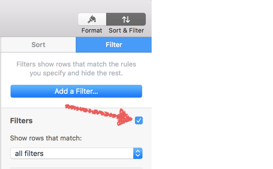
Meantime, Apple does provide a checkbox in the Sort and Filter panel to turn filtering on and off (see image below) and if you set both the filter and the SUMIF to use the hidden column proposed by SG, you can easily add a check box to toggle between SUM filtered and SUM all (example below).

Sort Filter checkbox: