Count unique dates within a date range

Dear Barry,

Thanks for your fast and detailed response. I understand how the formula works in general, it was simply that ”B” reference in the Condition argument. I thought ”B” referenced the whole column, not simply “this row“ in column B, as you Explained. I wonder if this is a fundamental misunderstanding I have had about how to reference variables in Numbers formulas.

I found this on help.apple.com:

So, if I understand you correctly, if the argument is supposed to be a single cell (I realize it can also be a text string), then the column reference with a single letter defaults to the cell in that column at the row containing the formula. Is that right? I just never saw that before in any of the documentation.

Incidentally, it seems to me that the sumif formula could get pretty burdensome the longer that column gets. It seems that an easier solution would be to sort the column first and then simply compare each entry to the one above, to see if there is a change. Something like this, perhaps?

IF((B2≠B1),B2,"")

Thanks again for your help. I am trying to learn this stuff and the documentation is a bit sparse.

Ultimately I am trying to duplicate the subtotals function from Excel. I know that I have to put my category totals in a separate table, but I will have a lot of categories that I want to subtotal financial amounts by. I don’t want to have to manually identify the categories because, they could be user ID numbers and could be in the hundreds (I need to total all donations, by donor, for a nonprofit application). I may resort to using Excel, but I wanted to see if I can to it in Numbers as a mental exercise.

Sorry for the long post. I realize now that I probably should have done this in a separate post, but I wanted to direct it to you because you understand this stuff and seem to be active. The only other posts on related topics were pretty old. I simply don’t know if it is possible to create a new post and then direct it towards a particular user to ask them if they can answer.

Best regards,

Chris

Barry,

I have a related question and you seem to understand this stuff pretty well.

In several other posts, I found the following formula for finding distinct values in a column:

If entries are in column B starting from B2

In C2 enter the formula:

=IF(COUNTIF($B$1:$B1,B)=0,B,“”)

and apply fill down.

I don’t understand this. It appears as is the countif call is using a partial column range range — say B1:B6 in cell C6 — to compare to a full column, B. How can you compare two ranges of unequal length?

Thanks for any insights.

Chris

Hi Chris

=IF(COUNTIF($B$1:$B1,B)=0,B,“”)

This is what the formula looks like in Row 2.

Let's move it down to Row 5, where it will look like this:

=IF(COUNTIF($B$1:$B4,B)=0,B,“”)

Note that the only change in the formula is the end of array reference to B4—the cell one above the row in which this copy o the formula resides.

COUNTIF accepts two arguments:

COUNTIF(test-array,condition)

test-array ( B1:B4 ) is the collection of values in the specified array of cells—in this case, the four values in B1, B2, B3 and B4.

condition ( B )is the single value which must compared with each of the values in the test-array. Each cell containing a value that meets the condition is included in the count.

In this case, the value, to be counted must equal (implied) the value in 'this row' of column B. Because Numbers knows a single value is expected for this argument, the row number does not need to be specified—Numbers will assume the value to be in 'this row', the row containing the formula.

IF the count is zero, there are no cells in column B above this row that match the value in 'this row of column B, and the count will be zero.

A zero count means this is the first time this value has appeared in the list, and the value in 'this row' of column B is copied into the cell containing the formula.

If the count is not zero, then this is not the first time the value has appeared in the list, and a null string ( "" ) is inserted in the cell containing the formula.

Regards,

Barry

Hi Chris,

Use of a letter-only reference targeting a single cell may not be noted in the documentation. I don't recall whether the possibility is something I discovered by accident, something I found by exploration, or something I picked up following a discovery by someone else. The logic behind it seems related to Numbers similar abiity to dump the not-needed parts of a full cell address:

=Sheet 3::Table 1::A1 is the full address for an example cell.

If the Table name has been changed from "Table 1" to a name not shared with any other table in the document, then a formula in a different table (on the same sheet or on another sheet) needs only the table name and cell coordinates.

If the table name is not unique within the document, then any formula on a different table (on the same sheet or a different sheet) must use the full address.

"All the cells in the column," circled in your note, can mean "All the cells in the column" or "All the cells in the column except those in Header rows or Footer rows," depending on the function containing the reference. This allows for formulas like SUM(A) in a footer row or Header row cell in column A without generating a self-reference error.

Regarding your Sort, then Compare suggestion: This would work, provided you added the formula AFTER doing the sort.

Sorting after adding the formula may produce odd results as Numbers tries to keep the reference on the 'same' cell in its new location. The need to edit after the sort and/or the need to collect the scattered distinct values after copying them o the new column may make this more clunky than the method earlier described, which detects and makes an unspaced list in one sweep.

Regarding your end goal:

It's not necessary to manually extract your categories. You can use COUNTIF (as above) to create an index column for a category, then use VLOOKUP or MATCH and INDEX to collect the list of distinct values onto a summary table, and use SUMIF to collect the total for each category.

As the devil is in the details, and the details are specific to the tables involved, I'd suggest posting what you want to solve as a new question.

Include the version number for the OS X/macOS you are using and the version number of Numbers you are using, plus screen shots from which the structure of your data can be seen.

Regards,

Barry

Hi moose,

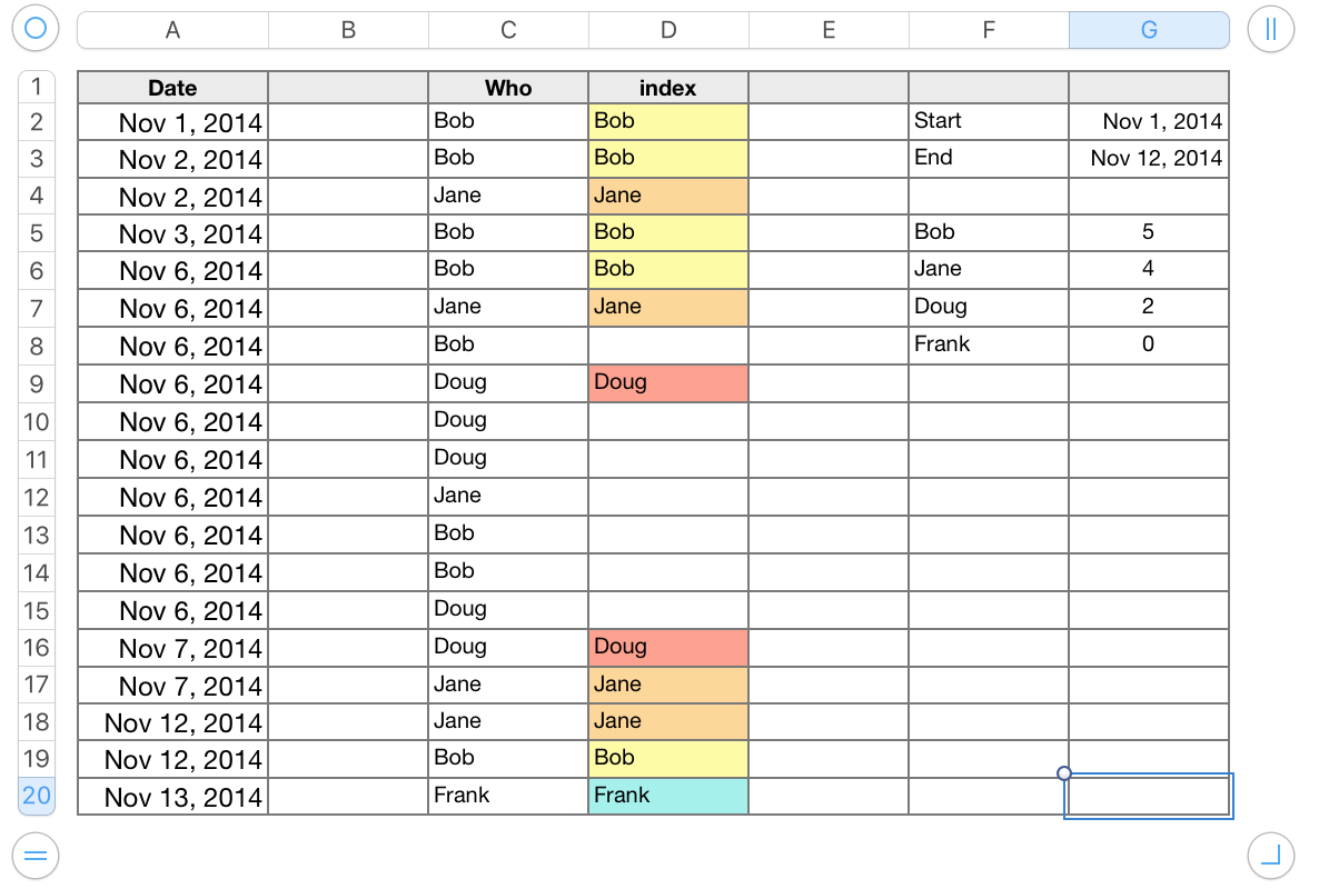
You want to count the number of distinct dates on for which there is at least one record for Bob, and to do the same type of count for each of the other individuals. The only unique dates on the table (and these are unique only within the context of column A of that table) are in Row 2 and Row 5. All other dates in the column occur at least twice.

This table uses an index column to hold the names to be counted. The highlighting isn't necessary; it's a visual check that I used to match the visual count with the calculated one in column G.

Two formulas are used, one to create the index values in column D, the other to perform the counts in column G.

D2: =IF(COUNTIFS(A$1:A2,A2,C$1:C2,C2)=1,C2,"")

COUNTIFs uses two test-values, condition pairs to determine the number of times this date-name pair has been entered up to this row in the table, and includes the row in the count only if both conditions return TRUE

• A$1:A2,A2: the date on the row (in the range A$1 to 'this row') is the same as the date in A2 ('this row of column A')
• C$1:C2,C2: the text on the row (in the range C$1 to 'this row') is the same as the text in C2 ('this row of column C')

The count is passed back to IF.

IF it is equal to 1, IF inserts the text (name) in 'this row' of column D, where it may later be counted.

IF the count is not 1, IF inserts a null string into 'this row' of column D.

The formula is filled down to the end of column D, and builds the list shown.

G5: =COUNTIFS(A,">="&G$2,A,"<="&G$3,D,"="&F5)

Here COUNTIFS uses three test-values, condition pairs. Again, all of these must return TRUE for a row to be included in the count.

• A,">="&G$2: The date in column A is on or after the date in cell G2
• A,"<="&G$3: The date in column A is on or before the date in cell G3
• D,"="&F5: The text (name) in column D is the same as the text (name) in F5 ('this row of column F')

The count is returned to the cell containing the formula.

The formula is filled town to the row containing the last name in the list of names in column F.

Further notes on COUNTIFS may be found in the Functions list, visible when = is entered in a cell on the table.

Regards,

Barry

HI moose,

Thank you for asking an interesting question.

Normally, I would keep the data (and the index column) on one table, but place the calculations in columns F and G on a separate 'summary' table. The data table needs enough rows to accommodate the data; the summary table needs only two columns and enough rows to hold the start and end dates, an empty row used as a separator, and one row for each person whose data is being summarised. All those empty cells below the sumamry rows are just wasted space.

Regards,

Barry

Barry,

This is very detailed and very clear.

Thanks for your advice and all your efforts.

Best,

Chris