Absolute Cell Reference for Range of Cells

Hi gb,

In the example, the Copy table cells reference the same cell in the Source table, using INDEX.

The formula entered in B2 is this:

B2: =INDEX(Source::$A:B,ROW(),COLUMN())

As the formula is filled across the columns, the column reference to A remains the same, and the column reference to B changes to match the column containing that iteration of the formula.

Specifying only the columns where a range is expected means the reference is to all cells in the column.

Fill the formula left to A2, then fill both down to row 3.

Adding rows or columns to the Source table and filling the new cells with data has no effect on the Copy table.

The Copy table must be enlarged using the Column and Row control handles at the upper right and lower left of the table, or the Column and row control handle at the lower right (visible in th first image, where only one table is selected)

As rows and columns are added, Numbers automatically fills the formula into the new rows or columns.

If the Copy table is extended beyond the size of the Source table, 'extra' columns or rows will contain a 'bad reference' error.

Adding rows to the source table removes the error in the previously 'extra' rows of Copy, because there the range, specified as the 'whole column' automatically sees the added rows.

The added column, though, must be deleted from Copy, then re-added to recopy the errorless formula in column C into column D.

Regards,

Barry

gabaroobrown wrote:

I would like to reference a range of cells from one sheet to another, all within the same spreadsheet. When grows and columns are changed in the source sheet,

Hi gabaroobrown,

I'm curious why you would want to do this. If you can post details, we may be able to suggest a more efficient approach to accomplish what you want to do.

BTW, I think you mean from one table to another, not from one sheet to another. The terminology is important in Numbers because the structure is a little different from other spreadsheet apps.

SG

HI gb,

Try this:

Master list table is named "Main", change to match your table name ('sheetname::tablename' if that tablename is used on more than one table in the document.

On the table for the email coördinator, use the model shown.

Table 2 contins this formula in A2:

=INDEX(Main::$A:$G,ROW(),MATCH(A$1,Main::$1:$1,0))

And the same formula in B2, but with a switch added to stop trying to retrieve names on rows betond the end of Main:

=INDEX(Main::$A:$G,ROW(),MATCH(A$1,Main::$1:$1,0))

Enter the formula for B2 in B2, Fill left into A2.

Fill both down to the end of Table 2 (which should be longer than Main).

For other report tables, use the same formula. Change the names in A1, B1 (and added columns, where needed) to match the name at the top od the column from which data is to be retrieved.

Regards,

Barry

Hi Barry,

I think you meant to post a different formula for B2, adding a "switch"?

SG

Oops!

Dinner was getting cold, and I was being called. 😊

Here's the correct formula, with the switch added:

=IF(ROW()>ROWS(Main::A),"",INDEX(Main::$A:$G,ROW(),MATCH(B$1,Main::$1:$1,0)))

"Cut off switch" part in bold, the rest is the same as the formula in A2, filled one column to the right.

Regards,

Barry

Final(?) revision:

Here is a model showing the Main tale, containing all the data, and three 'break-out' tables that collect the data needed for the name-badge maker, the email coordinator, and the birthday card sender.

'Name & email' contains the original 'unswitched' formula in column A and the 'switched version in column B. These are the two formulas shown above.

When making a final version of this tabe, use the formula below, in place of the two previously mentioned.

'Name only' contains the same formula (switched) with one revision—an absolute reference to column A in the 'switch' to ensure that ROWS() is always counting a column that it on the table. This is the formula shown below, and the one that should be used in all of these tables.

'Name & Address' contains the same formula as 'Name only', entered in A2, then filled down and right to the last row and column of the table.

Formula:

=IF(ROW()>ROWS(Main::A),"",INDEX(Main::$A:$G,ROW(),MATCH(A$1,Main::$1:$1,0)))

Apologies for the extra posts required to tidy up the small errors.

Thanks to SG for noticing I'd posted the 'unswitched' version twice above.

Regards,

Barry

One of the problems (maybe the only one) is that you have an extra = in front of the formula. In the formula editor you shouldn't see the =. With the formula displayed in the formula editor try deleting the leading =.

SG

Hi gb,

As SG has noted, the first error is the added = sign. The first = typed opens the formula editor, which displays ƒx to indicate this is a formula. The editor box will not display this =.

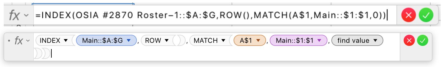
Here are three images of the formula editor. The first shows your start at constructing the formula using the mouse (or trackpad), the second your (unfinished) edit of my formula, copied and pasted to your table, and the third my 'unswitched' formula from cell A2 of the two column table in my post showing only two tables.

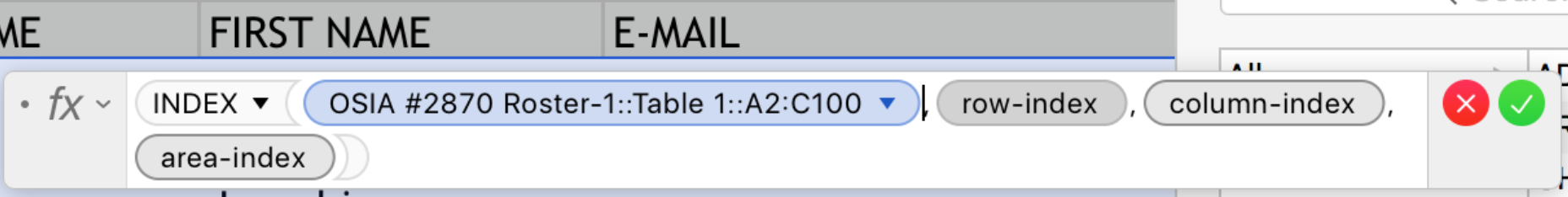
One advantage to building the formula references using the mouse is that it automatically includes as much of the cell or range address as needed. Here the blue lozenge shows a reference to the range of cells A2 to C100 on the table named "Table 1" on the sheet named "OSIA #2870 Roster-1".

In the copy/paste/edit version Upper of these two images), the first instance of the table name "Main" has been replaced with the sheet name "OSIA #2870 Roster-1", and no table name has been entered.

For a cell reference:

to a cell or range on the same table as the formula, Numbers needs only the address* of the cell.

to a cell on a different table from the formula, but on the same sheet, the name of the Table must be included.

to a cell on a table on a different sheet from the formula, the name of the Sheet must also be included.

(If no other table in the document has the same name as the one containing the cell, the Sheet name
may be omitted.

(range reference requirements are similar)

*"address" can be the full column&row address, of may include only the column letter. If only the column letter is used, Numbers will interpret it to mean "all cells in column X", "all cells not in Header or Footer rows in column X", or "the cell on 'this row' of column X", where 'this row' is the row containing the formula.

Both "Main" references should be changed to the same table.

"tablename::A2:C100" in your has several consequences:

• Row 2 of the Table is row 1 of the indexed area, so a row index generated by ROW() in cell A2 of the table containing the formula will return data from row 2 on the indexed area (which in row 3 of the Table containing the data. The list supplied to the email manager will start with Aiello, not with Adams.
• Even if the C100 reference is made absolute ($C$100), this reference will adjust when rows are removed from the table or when rows are added to the table between row 2 and (currently) row 100, the row may not adjust to include rows added to the end of the table.
• While the email list table requires data from only the first three columns (A,B and C) of the main table, setting these three into the formula means the range will have to be edited whenever the formula is used for a different table requiring data from later columns.

Changing the range reference to an absolute columns only reference covering all columns of the table eliminates these concerns:

• Row 2 of the table (where the data starts) is row 2 of the indexed area, and data will be returned to the same row of the table containing the formula as it is in on the data table (Main).
• Specified using only the Column references, the indexed area always includes all the rows of the data table.
• Setting the range to include columns A to the last column of the table, and omitting the number parts of the beginning and end addresses allows the same formula to work on any table pulling data from the Main table with no changes to the formula.

Suggestion:

• Rename "Table 1" (on the OSIA sheet) "Main"
  • click on the table
  • open the format inspector and choose the Table inspector
  • check the Table name checkbox to show the table name
  • double click the name and edit to "Main"
• Copy my formula (either the switched or unswitched version) from this discussion

  (do not include the = sign)

• Select (one click) cell A2 on the names and emails table on Sheet 2 of your document.
  • Press delete to delete the current contents (the formula in your pot above)
  • Type = to open the Formula editor.
  • Paste

You should see the formula you copied from here, displayed in format showing that Numbers has accepted it as a formula.

If so, click the green checkmark to confirm it, and check the see that it has provided the expected result.

If so, you can rename your data table (currently "Main") to the name of your choice. Numbers will automatically revise the formula to match the new name.

Fill the formula into the rest of the rows and columns on the Names and email table.

Regards,

Barry

Your screenshot shows F instead of IF at the beginning of the formula. Try adding that missing I.

SG

Hi gb,

I think SG may have tried to view the screen shot without magnification. This is the only formula shown in the screen shot, and the I of IF is definitely there.

Possible causes for the syntax error:

• The character between ROWS and Main::A appears to be a pipe ( | ) or upper case I. It should be an opening parenthesis — ( — shown in bold in the copy of my formula below the screenshot.
• Check all of the commas. They're too fuzzy to see clearly in the screen shot. If one is a period, it will cause a syntax error.

fx IF(ROW()>ROWS(Main::A),"",INDEX(Main::$A:$G,ROW(),MATCH(B$1,Main::$1:$1,0)))

"Double checking on terminology: Sheet is my entire file (in this case named Master List or some such). Each tab takes me to a different table within the sheet, right?"

Not quite.

• "Spreadsheet" or "Document" or "Spreadsheet Document" is the entire file.
• Each Tab takes you to a different Sheet. A Sheet may have one Table, more than one Table, or no tables at all.
  • Unless you have added a Table, Duplicated a Table, or split a Table into two tables (or more), each of the Sheets in your Document will have one Table.
  • Unless you have renamed a Table, the original Table on each of the Sheets in your Document will have the default name "Table 1"
  • You will not see the Table name (green arrow) unless you have checked the "Table Name" box (red arrow) in the Table Inspector.

• Changing the name on a Tab changes the Sheet name, but has no effect on the table name. You have changed the name of the Sheet containing the Table containing the cells and columns referenced by the formula above, but I suspect you have not yet renamed the Table. Do this before you fix the syntax error in the formula.
  • To rename the Table, click on any cell in the table to select it, Open the Format inspector, and choose Table.
  • Check the Table Name box to show the Table name.
  • Double click the name, then edit it as you would any other text.
• With the Table renamed to "Main" the formula (with the syntax corrected) will be able to find the table.

"My understanding is that:

INDEX(Main::$A:$G,ROW() means I'm referring to table "Main, Columns 1- 6 (A - G), any row

MATCH(A$1,Main::$1:$1,0) means .... well, it is trying to match to position of where the items are, right?"

From the Function Browser:

The INDEX function returns the value in the cell located at the intersection of the specified row and column within a collection of cells…

INDEX(range, row-index, column-index, area-index)

• Main::$A:$G is the range, the "collection of cells"—all of the cells in columns A (1) to G (7) of the Table named "Main"
• ROW() provides the number used as the row-index. The row and column indices start at the top left corner of the range (cell A1 of Main) and count down and right from there. ROW() returns the number of the row that it is in, so in Row 2 of the receiving table, ROW() gives INDEX the value 2, and INDEX will return a value from Row 2 of Main.
• MATCH(A$1,Main::$1:$1,0) provides the number used as the column-index.

From the Function Browser:

The MATCH function returns the position of a value within a collection.

MATCH(search-for, search-where, matching-method)

• search-for the value in A$1.
• search-where: Search in Main::$1:$1 (Row 1 of the Table named Main)
• matching-method: 0 means "Find the exact match"

In my email manager example, the value in A1 of the table with the formula is "Name". Match finds Name in the first cell of Row 1 of Main, so the column index is 1. The value in B1 of the table with the formula is "email", which MATCH finds in he sixth cell in Row 1 of Main, so in column B, INDEX's column-index is 6, and the formula returns the email addresses from column 6 of Main.

You'll find descriptions (and at least one example) for each function supported by Numbers in the Function Browser. Open the browser by clicking any (empty) cell in a table and typing =. Click on a category to find all functions in that category, or type the first few letters of a function name to locate that function.

Regards,

Barry

Barry wrote:

I think SG may have tried to view the screen shot without magnification. This is the only formula shown in the screen shot, and the I of IF is definitely there.

I'm not a big fan of the recent configuration of how forum software displays posts. Anyway, here is what I see on my end: no I in the IF:

SG