How to use a tick box to change a field’s colour in Numbers 09 on MacOS high sierra

Hi BlackyNeo,

You can use conditional formatting, BUT…

Conditional format rules depend on comparing the value in the cell to be formatted with either a fixed value, written into the rule, or the value in another cell, referenced in the rule.

HD's 'conditional highlighting' suggestion can work, but will require two tables: one to hold the data (and the checkboxes), the other, identical in size and shape to the group of cells (rows) to be formatted, to hold the cells to be formatted according to the checkboxes.

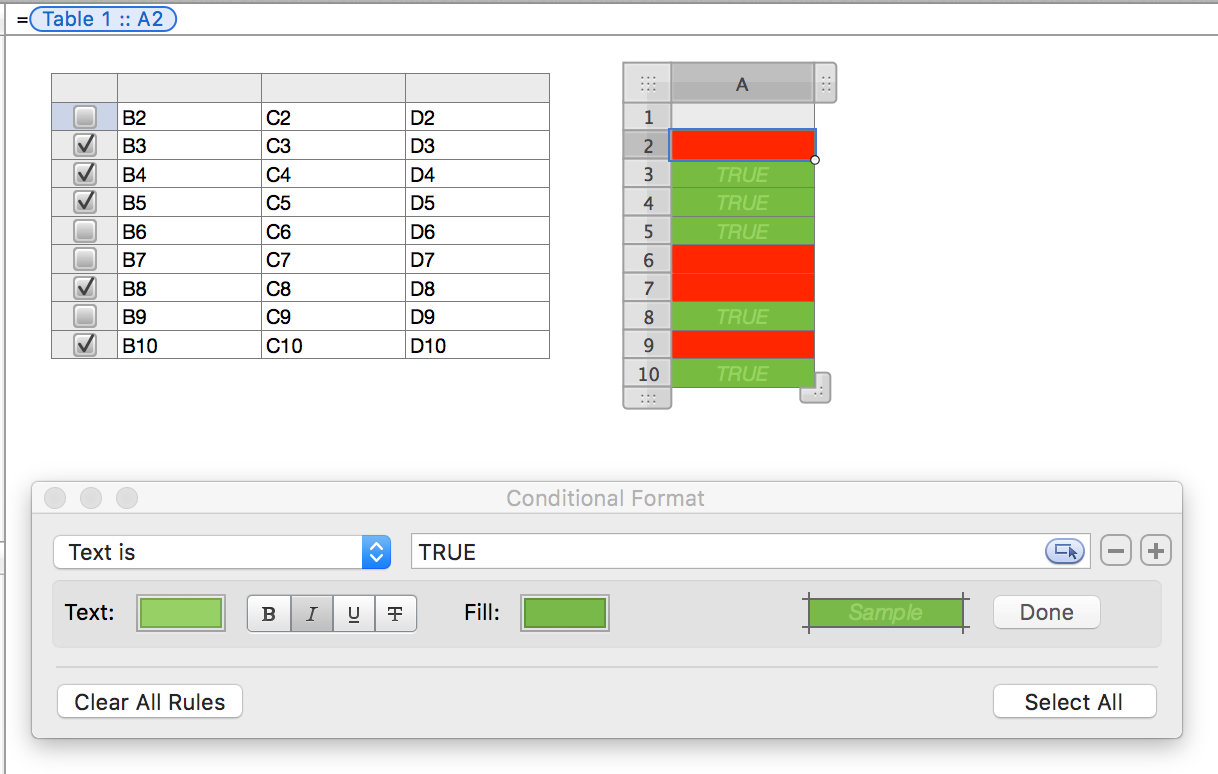
Here are the two tables. Table 1 on the left contains the data. Table 2, on the right has a single column of cells.

Cells A2 to A10 in Table 2 are formatted with red fill and red text.

The cells are selected, and the conditional formatting rule below the tables has been applied.

(I used a slightly lighter shade of green for the text than the fill to make the text visible in the image. In the 'finished' view below, the text and fill colours match.)

The formula in Table 2::A2 is shown in the entry box above the tables. The formula is filled down to row 10.

To highlight the cells on Table 1, it is necessary to remove the Fill Colour from Table 1, and do three things with Table 2:

• Select Table 1, then choose the graphic inspector and set the Fill to none.
• Select Table 2, resize to match the width of columns B to D of table 1 (or to match the full width of Table 1).
• Sent to Back, using the Arrange menu.
• Slide it under (behind) and align it with Table 1, using the arrow keys (and Shift).

Result:

Regards,

Barry

BlackyNeo wrote:

i need to create a tick box that will allow a cell (or preferably row) to change colour if true.

If you're willing to use Numbers 4 or 3 (something you're going to have to do any as Numbers 2, part of iWork '09, is "orphanware" and sooner or later is not going to work well) then all you have to do is a short script like the one below to highlight a row.

1. The first time, make sure 'Script Editor.app' is checked at System Preferences > Security & Privacy > Privacy > Accessiblity.
2. Copy-paste script into Script Editor (in Applications > Utilities).
3. Change the color "red" to whatever you want and change column number if needed.
4. Click anywhere in the table.
5. Click the triangle 'run' button.

It's time to upgrade your Numbers!

SG

set checkboxCol to 2 -- column "B"

tell application "Numbers"

tell (front document'sactive sheet'stable 1 whose selection range'sclass is range)

repeat with r in rows

tell r to if cell checkboxCol's value is true then set cells 1 thru -1's background color to "red"

end repeat

end tell

end tell

Hi BlackyNeo

You can use conditional highlighting:

My checkbox is in B2, and I have set C2 to the value of B2:

so C2 will switch from TRUE to FALSE depending on the state of the checkbox.

I select C2 and in the Cells inspector click Show rules... next to Conditional Format:

Set up two rules:

Green text and green fill when the text in C2 is TRUE, Red text and red fill when the text in C2 is FALSE

Close the Conditional Format panel. Ticking and unticking the checkbox will change the colour of the C2:

C2 can be filled across to give a coloured row.

What you can't do is type data into C2 - this would override the two rules and the formatting will revert to black on white.

Hope it helps,

H

Hi BlackyNeo,

Numbers 2.3 (Numbers'09)

The table on the right (Table 2) has this formula in cell A1 (filled down and filled right)

=IF(Table 1 :: $A1=TRUE,Table 1 :: B1,"")

If the checkbox is ticked, make this cell equal to Table 1 Cell B1, else insert "" (NULL)

Conditional Formatting for Table 1 Cell A2 B1

It is a long time since I was familiar with Numbers '09. Perhaps another user will reply with a quick and easy way to fill that Conditional Formatting to all cells in Table 1. I had to do it cell by cell 😊.

Regards,

Ian.

Edit: Hide (Cut and Paste) Table 2 on another Sheet. Ian

You can't control the color of a cell or row via a formula. You can control it via a script. However, it appears that you are using nearly a decade-old version of Numbers, whose scripting support is less robust. So I hesitate to suggest a script.

SG

I'm a bit less hesitant than SG so here's a script that will run in Numbers 09 (and later versions I would have thought, but not tested):

tellapplication"Numbers"

telldocument1

tellsheet1

try

set active_table to first table whose selection range's class is range

on error number errnum

if errnum = -1719then-- nothing selected

display dialog"Select at least one cell in the table before running this script."buttons {"OK"} default button1giving up after10

return

end if

endtry

tell active_table

ifvalueofcell"B2"isfalsethensetbackground colorofcell"C2"to {64634, 467, 1798}

ifvalueofcell"B2"istruethensetbackground colorofcell"C2"to {32896, 65533, 2034}

endtell

endtell

endtell

endtell

The checkbox is in cell B2. Running the script will change the colour of C2 depending of the state of the checkbox.

Pro: You can edit the data in C2 without affecting the colour fill.

Con: You have to run the script to change the colour fill.

Cheers,

H

Yellowbox writes:

"Perhaps another user will reply with a quick and easy way to fill that Conditional Formatting to all cells in Table 1. I had to do it cell by cell 😊."

Easier, and a bit quicker, but not "quick and easy."

The conditional formatting rule can be applied to all cells on the first table at the same time, but each of those rules will reference the same cell on the second table.

So after applying the rule, you'll need to go through the cells one by one and edit the cell reference in the rule to match the correct 'partner' cell for the one to which the rule is to apply.

Not a lot quicker.

Regards,

Barry