Hi limmy
With the numbers w a y o v e r on the left and no connecting lines between them and the cells in column L, it's difficult to keep track of where the mentioned cells are, and what should be/is in them.
L35 is the sum: (24.75)
In L40 the result ( 4.00) is given. (What is this the result of?)
But it happens that the result hat (has?) figures behind the point.
Now I would like to have a formula which definitely has a whole number without anything after the point.
(The numbers following the decimal are all zeroes in L40 and in M40. If this is always the case, then your result here is already a whole number, and you need only change the Format of the cell to Number, 0 decimal places using the Format Inspector.)
and the rest shall be seen in row L44. (What is "the rest"?)
The formula in column L shall divide into by 6 and in column M /4. (What is being divided in these two cells?)
(The result in L40 implies the value in L37 (25.25–not mentioned in your description) is divided by 6 then rounded down to the nearest whole number (and presented with two places after the decimal to match the format of the numbers in the rest of the column.)
Assuming those guesses are correct, Here's a possible set of formulas. The image is of a section of your table showing the cells involved in the formulas.
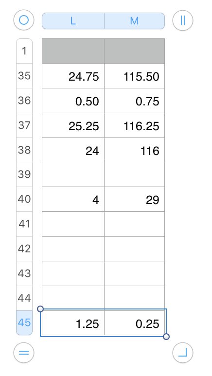
L37: (Assumed) This cell contains the sum of L35 and L36.
L38: The number above, rounded down to the nearest multiple of 6:
L38: MROUND(L37−3,6) M38: MROUND(M37−2,4)
MROUND rounds a number to the nearest multiple of another number. The rounding will be up or down, depending which multiple is closest. the -3 (half of 6) and -2 (half of 4) are offsets that force the result to the nearest multiple less than (or equal to) the number in L37. Format the cell to show two decimal places if desired.
L40: INT(L37÷6) M40: INT(M37÷4)
INT returns the integer portion of the result of the expression in the brackets, and ignores the fractional part
L45: L37−L38
Regards,
Barry