Conditional formatting/rules for working out VAT

Hi Patrick,

The error message is pretty straightforward.

The formula in this cell is IF(LEN(B2)<1,"",H2÷("1."&RIGHT(B2,2)))

The part in bold is the trouble point, not because of an error in the formula, but due to 'bad information' in B2.

Like the pop-up menu items in the Expenses table, the ones in column B of this table need to be edited to include the VAT rate as the last two characters of the item.

B2 is set to "Accommodation", so the RIGHT in bold picked up the last two characters "on" from Accommodation. The concatenation operator attached these two characters to the 1. in quotes before that making the text string "1.on".

/ (displayed in the formula as ÷ ) said 'I can't divide 100 by 1.on' and threw an error message saying that.

Edit the pop-up menu items in column A to 'Accommodations 07' 'Taxi 18' as shown in my earlier post, and all should be well.

Regards,

Barry

Hi Patrick,

I've assumed your description of VAT rates is complete: All products you handle are subject to VAT, "Accommodation" at a rate of 7%, ALL other products at a rate of 18%, and VAT is deducted from the listed price.

VAT is calculated in column I using the formula shown below the table (and copied here):

I2: IF(LEN(B2)<1,"",IF(B2="Accommodation",H2×0.07,H2×0.18))

Net, in column J, is calculate with this formula:

J2: IF(LEN(I2)<1,"",H2−I2)

Each formula is entered in the indicated cell in row 2, then filled down to the end of the column.

The core part of each formula is shown in bold. That part is enclosed in each case by a 'switch' that prevents the calculation from occurring until there is an entry in column B (for the VAT calculation) or a result in column I (for the Net calculation). See the examples in row 6 of the table.

I would suggest using a pop-up menu cell (with 'none' as the first item) for each row in column B to ensure consistent spelling of Accommodation, required to activate the 7% rate in column I.

Regards,

Barry

Hi Patrick,

When the list of exceptions and discounted rates gets longer, and with more categories, the formulas get more complicated and error prone. With four categories (18%, 7%, 5% and 0%) you're at the point where I would switch from IF to a lookup table, or would include the rate as the last part of the product name, as you've done in your latest example.

A question arising from your new example:

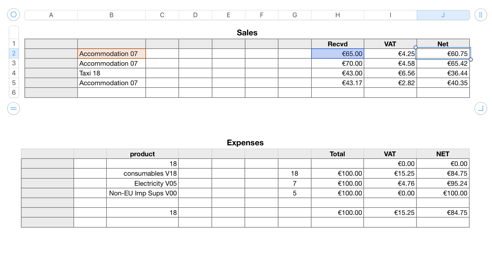
All three amounts listed are 100.00

Reading from the bottom up…

The third, with a VAT rate of 0% is obviously correct - the VAT is 0 and the net amount paid is the same as the total amount paid.

The second, at 5% shows the VAT amount as €5.00, which is 5% of the total amount (100.00).

But the first, at 18% shows the VAT amount as €15.26, which is 18% of the Net paid amount (84.74), not the Total amount, for which 18% would be €18.00.

I suspect that one shows the correct calculations: The VAT, like the GST here, is added to the base price, and the result is the Total paid. The examples below work back from the Total to determine the net and VAT at the percentage rate applied to that net amount.

^^^^^^^^^^^^^^^^^^^^^^^^^^^^^^^

Here is the first example again, with calculations based on the assumption that the VAT is calculated by adding the specified percentage to the base (net) price.

The second example, placed directly below the first, uses the same assumption, and the same formulas, differing only in their references to column B (top) or column C (bottom) to collect the VAT rate applicable to that transaction, and in the column used as a trigger for the switch (described earlier).

Sales::J2: IF(LEN(H2)<1,"",H2÷("1."&RIGHT(B2,2)))

Expenses::J2: IF(LEN(C2)<1,"",H2÷("1."&RIGHT(C2,2)))

Sales::I2: IF(LEN(J2)<1,"",H2−J2)

Expenses::I2: IF(LEN(J2)<1,"",H2−J2)

All formulas are filled down from Row 2 to the last row of the table.

A note regarding the first example: Calculations on the table in the first example assumed the VAT rate was applied to the TOTAL price, and was deducted from the TOTAL amount to produce the Net amount.

The calculation in rows 2 and 4 of that table is correct for those assumptions. The calculations in rows 3 and 5 use the 18% VAT rate as I neglected to correct the spelling of Accommodation in the formulas in those rows.

Regards,

Barry

Hi Patrick,

The pop-up menus are easy to create.

Make a full list of the items in a handy column, one item to a row.

Check the spelling of all of the items and correct if necessary.

Make sure that the last two characters of the item express the VAT rate in percent for that product. Include a leading zero for rates under 10%. (do not include the % sign)

When you have the complete list, select all cells containing the items , then, in the Format inspector, choose Pop-up menu as the format and choose Start with Blank from the pop-up below the list.

Each of the selected cells will then be a pop-up menu containing all of the listed items. Set one of them to 'none' (displays as a blank), copy the cell, then paste it into all the cells where you need it.

Regarding error triangles:

What is the error message? (click the triangle to open a message box. Select and copy the message and paste it here.

Also copy and paste the formula (from the editor)

And a screen shot with the cell containing the formula selected, and including the cells highlighted when that cell is selected. Could also be shown with the Formula editor opened to show the formula, then dragged down to reveal the selected cell as well. (See example in my first reply).

Regards,

Barry

Hi Patrick,

Sales:

I don't see the error messages.

The one for the selected cell (I2) is likely "Cell J2 contains an error", since I2 depends on the contents of J2.

What is the error message (and the formula) in J2? To read the message, click once on the error triangle. Copy the message, and paste it here.

Expenses:

C3: This menu item needs 00 at the end, not just a single 0.

The column to the left of Total on my table is not necessary, nor is its content. Just there as a reminder to me of the rates on that row.

Regards,

Barry