Hi Marc-André,
I'm assuming the reference "an example of a table can be seen at the end of the following link" referred to this pair of tables:
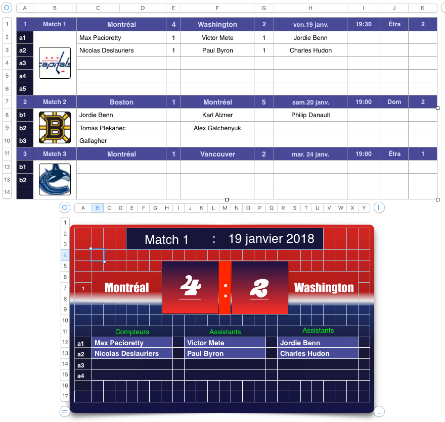
Going on that assumption, I did a reconstruction of (parts of) the Data table at the top and the Game table below it, using those names for the two tables.


As I read your question, your concern is getting the names of the Montreal goal scorers and those credited with assists on those goals for a specific game.
The tables show my results for Match 2.
Changes made to your tables:
Data:
I changed the a1, a2, a3 style of labels in column A of Data (and column A of Game) to numerical values calculated (in the Game table) from the Match number, entered in A7 and the position of the row in relation to A7.
The corresponding numbers in Data were entered by hand, but could be calculated using a similar formula using the match numbers entered in the top row for each game.
I note there is a column reference tab for column D in this table, but no sign of that column in the visible part of the table. I included a column D in my version, but did not enter any data in it. This 'phantom' column may affect results of the formulas when copied to your table.
Game:
See note above regarding numbering of the 'goal' rows.
Formulas:
Data: This table currently contains no formulas. All data is entered directly. As mentioned above, It should be possible to use a formula in column A to calculate the 'goal line' numbers from the match numbers at the top of each match.
Game:
A11: A$7
This copies the match number, entered in A7 to the top row of the game number.
A12: IF(ISERROR(MATCH(100×A$7+(ROW()−11),Data::A,0)),"",100×A$7+(ROW()−11))
The core formula, in bold, calculates a reference number for each row where the goal scorer and assists are to be Shown.
The calculation is done twice. The first result is given to MATCH, which searches for that value in column A of Data. If the number is not present in that column, MATCH returns an error, ISERROR returns TRUE, and IF inserts a null string in the cell (see A17 and A18 of Game). If the number is present, MATCH returns a number corresponding to its position in the column (which is ignored), ISERROR returns FALSE, and IF jumps to the second copy the calculation which places the number in the cell.
The formula is filled down to the last 'Goal line' cell in Game::A, A18.
B12: IF(LEN($A12)<1,"",VLOOKUP($A12,Data::$A:$K,3,FALSE))
J12: IF(LEN($A12)<1,"",VLOOKUP($A12,Data::$A:$K,6,FALSE))
R12: IF(LEN($A12)<1,"",VLOOKUP($A12,Data::$A:$K,8,FALSE))
Again, a core formula in bold and a switch to turn it off enclosing the core part.
IF checks for content in 'this row' of column A, and inserts a null string in its cell if none is found. If there is content, IF passes control to the core formula, which gets the value from 'this row' of column A, searches for it in column A of Data, and returns the value from third, sixth or eighth column of the row where it finds that number. The FALSE argument means VLOOKUP will not accept a 'close match' with the search value.
The three formulas would normally be filled down their respective columns to row 18, but cannot be filled down because they are in merged cells. This alternate process will work, though:
- Enter the first formula in B12. Confirm the entry with the green checkmark, then Copy the cell.
- Click on J12, and Paste.
- Click on R12, and Paste.
- Click twice on J12 to open the Formula Editor, and change the 3 to a 6. Click the green checkmark to confirm.
- Click twice on R12 to open the Formula Editor, and change the 3 ot an 8. Click the green checkmark to confirm.
- Click on B12, Copy. Shift click on B18 to extend the selection to B12:B18. Paste.
- Click on J12, Copy. Shift click on J18 to extend the selection to J12:J18. Paste.
- Click on R12, Copy. Shift click on R18 to extend the selection to R12:R18. Paste.
The zeros in rows 15 and 16 (and the second assist cell of row 13) are the result of VLOOKUP returning a value from an empty cell. They are avoided in row 14 (Gallagher, unassisted) by typing a space in the corresponding cells in the Data table.
Do these address what you are trying to accomplish here?
Regards,
Barry