How to use the if and or functions with a drop down menu to calculate specific values.

Hi Kaliber,

What you are attempting to write is a set of nested IFs.

Your pop-up menu has three items: Item A, Item B, Item C.

(I use letters rather than numbers here to visually distinguish between the choices and the results.)

The syntax for IF is: IF(if-test,if-true,if-false)

if-test may be any expression that returns a boolean result, either TRUE or FALSE.

if-true tells Numbers what to do if the expression returns TRUE

if-false tells the formula what to do if the expression retruns false.

In your case, the first IF tests if the first item in the pop-up menu has been chosen.

If that expression returns TRUE, then the if-true part returns the value 100, and the formula is exited.

If that expression returns FALSE, the next value is tested for by the second IF.

Here's what it looks like. The Pop-up menu is in cell A2, the nested IFs formula is in B2, and "the formula" (named in your question) is in C2:

B2: IF(A2="Item A",100,IF(A2="Item B",50,IF(A2="Item C",220,0)))

C2: 1000-B2

Regarding the "etc., etc… part:

Although you could continue with additional nested IFs, each included as the if-false part of the previous IF, this soon be comes cumbersome, prone to error, as difficult to troubleshoot. For me, three is pretty much the limit. Beyond that (and even for a three item example), I'd turn to a lookup table and either VLOOKUP or a team effort by MATCH and INDEX to do the job.

Here's the same example, this time using VLOOKUP, and adding three 'etc.s' to the menus:

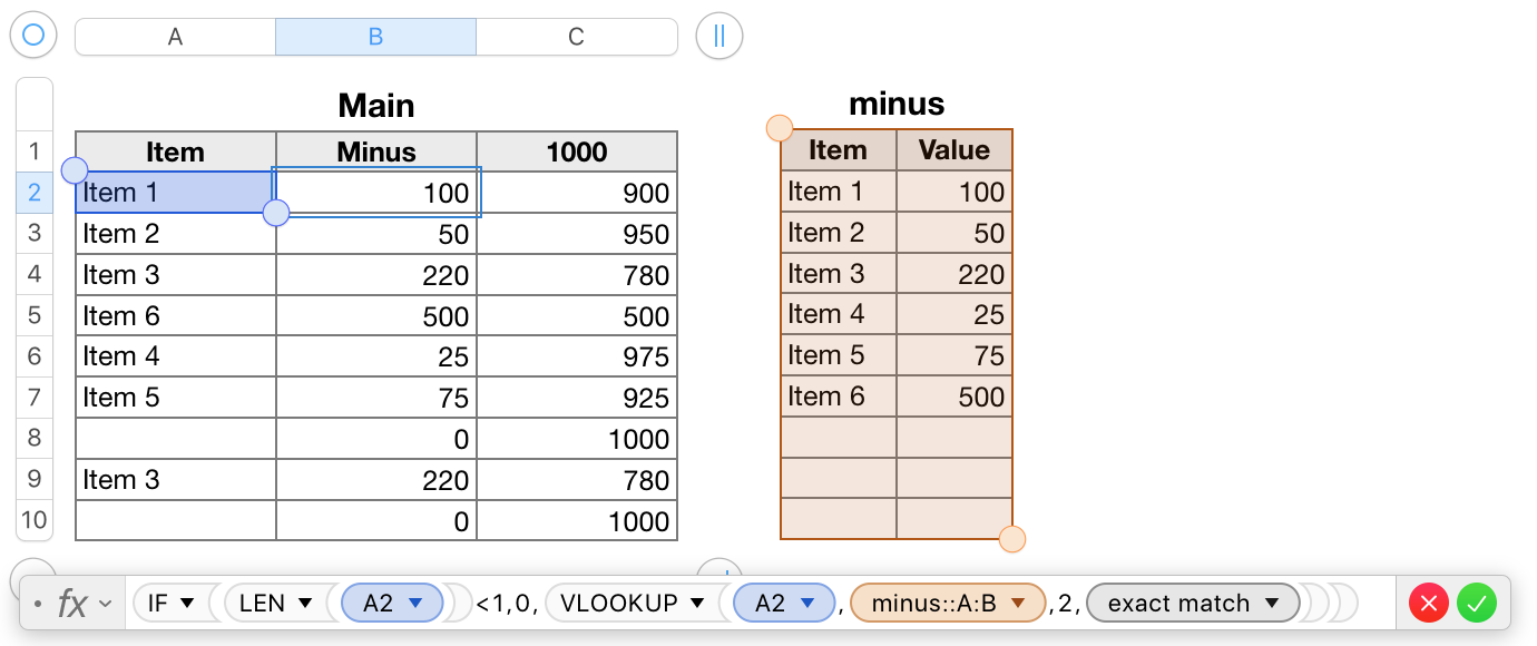
The formula shown below the tables is entered in the selected cell (C2) of the "Main" table, and filled down to the end of that table.

The popup menu cells were created by this process:

• Enter the menu choices, one per row, n the order you want them to appear in the menu, in column A of the lookup table, "minus"
• Select the cells containing the menu items list (minus::A2-A7).
• Click the Format brush to open the Format Inspector, then choose Cell.
• Use the Data Format pop-upmeu in the inspector to change the cells' data format to Pop-up menu.

Each of the selected cells, A2-A7 in the table 'minus' is now a pop-up menu, containing the list of menu items in those cells.

• Select cell A2 (one click), then chence the pop-up menu below the item list in the Inspector from 'Start with first item' to 'start with blank'.
• Set the pop-up menu in A2 to 'none' (which displays as a blank), then Copy (command-C)
• After copying, set cell A2's menu back to 'Item 1'

Now, move to the Main table.

• Click once on cell A2 of Main to select it.
• Shift-click on the last cell in column a to add it and all cells between it and cell A2 to the selection. Paste (command-V)

Each cell in the selection now contains a copy of the pop-up menu. All the cells are set to 'none'.

Column B:

Enter the formula below in B2, then fill it down to the last row of column B.

B2: IF(LEN(A2)<1,0,VLOOKUP(A2,minus::A:B,2,FALSE))

The part shown in bold is the core formula that looks up the chosen Item value in column A of 'minus' and returns the corresponding value from column B (column 2) of the same table. The FALSE argument at the end tells VLOOKUP to accept only an exact match between the menu choice and the list in column A of 'minus'.

The IF part of the formula returns a zero if no choice has yet been made (or if 'none' has been chosen) in that row's pop-up menu in column A. If any item (other than 'none' has been chosen, the LENgth of that item will be 1 or more characters, the if-test will retrun FALSE, and IF will call the core formula to do the lookup on that value.

To add more 'etc.s', you need only add more items to the pop-up menus, and to the list in column A of 'minus', and add the corresponding values to column B of 'minus'.

Regards,

Barry

You could use something like this:

Create a table (I named it "Dropdown" in this example):

Where the first row is a header row and the first column contains each entry in the pop-menu. The second column should contain the values that correspond to each dropdown entry.

In another table where "the formula" reside do something like this:

"The formula" in my example is "2*B2". In cell B2 I entered the value "100"

in cell C2 I entered the formula:

=2*B2+VLOOKUP(D2, Dropdown::A:B, 2, 0)

you can change "2*B2" to whatever your formula is

shorthand for this is:

C2=2*B2+VLOOKUP(D2, Dropdown::A:B, 2, 0)

Kaliber554 wrote:

Hello all! I'm trying to write a formula where, when I select from a drop down a specific value will be tied to that value. Example!

I select drop down 1, it subtracts 100 from the formula
I select drop down 2, it subtracts 50 from the formula
I select drop down 3, it subtracts 220 from the formula etc. etc...

You also have other options that avoid the need for extra tables or getting tangled up in nested ifs.

If you're just picking a number from a Pop-Up Menu.

Then you can use a simple CHOOSE function.

=CHOOSE(A2,−100,−50,−220)

If you are choosing more complex values from a Pop-Up Menu:

Then you can do something like this:

=CHOOSE(MATCH(A2,{"Dropdown 1";"Dropdown 2";"Dropdown 3"}),−100,−50,−220)

Substitute ; for , in the formulas if your region uses , as a decimal separator.

SG

Assumptions regarding the two row table:

A2 contains the Gross Profit amount. The formula shown below the table is in J2, and is intended to calculate the Net Profit.

For this to happen, all of the values in A2 to I2 must be numbers (and may be formatted as numbers or as currency).

That means the formula shown will not work with I2 containing a text value, as shown in your example. SUM will not complain with an error message, but will assign a number value of 0 to the text in I2.

If you do not need to display the reduction in Net Profit due to the choice of Inverter, you can edit the formula shown in your post to include the VLOOKUP or CHOOSE formula that calculates that amount.

If you do need to show the amount by which the inverter choice reduces the Net Profit, then you will need to provide a cell for that display and one for the pop-up menu in which the choice is made.

Showing calculated Inverter amount:

Not showing Inverter result:

The same is true using SG's CHOOSE formula. Place it in I2 I2 if you need to show the Inverter amount; us it to replace the VLOOKUP section of the last formula above if you do not need to display the Inverter result.

Regards,

Barry

PS: costs in B2 through H2 are all set to 1 fo the example.

B

You can try something like this:

The formula in J2:

=$A2−CHOOSE(MATCH(I2,{"SE3000H-US","SE3800US","SE5000H-US","SE6000H-US","SE7600H -US","SE10000H-US"}),−100,−200,−300,−400,−500,−600)

SG