Get value by selcting 2 checkboxes row/column

SGIII is correct about testing with the core formula, then adding the bells and whistles. In my example, the core formula (in Table 2::B2) is this part:

INDEX(Table 1::A16:C20,MATCH(TRUE,Table 1::A16:A20,0),MATCH(TRUE,Table 1::A17:C17,0),area-index)

IF(AND(COUNTIF(Table 1::B2:C2,TRUE)=1,COUNTIF(Table 1::A3:A4,TRUE)=1),INDEX(Table <<<line break inserted to match

1::A1:C5,MATCH(TRUE,Table 1::A1:A5,0),MATCH(TRUE,Table 1::A2:C2,0),area-index),"xx")         alignment in your image above

comparing your pasted formula to the one I copied directly from the formula editor for that cell. I don't see any differences. Yu could try deleting the ,area-index part I've shown in bold italic above. If that doesn't cure it, I'd guess that you live in a region where the , is the decimal separator, and need to change the list separators in the formula from , to ;

Here's a copy/paste able version of the formula, revised for regions other than North America.

IF(AND(COUNTIF(Table 1::B2:C2;TRUE)=1;COUNTIF(Table 1::A3:A4;TRUE)=1);INDEX(Table 1::A1:C5;MATCH(TRUE;Table 1::A1:A5;0);MATCH(TRUE;Table 1::A2:C2;0));"xx")

Regards,

Barry

Hi d,

This looks like 'embedded tables' on a large grid, ala MS Excel. In the Numbers model, each of those groups of cells would be a separate Table, containing columns A, B and C, and Rows 1-4 (or 1-5 for the one with three rows of number choices). Placing them on a single table isn't impossible, but it does change the way the formula has to be written.

Note that the 'full row' and 'full column' references have been replaced with references to a specific range of cells in a row, a range of specific cells in a column, and a specific range of cells in a rectangular array. (To shorten the overall formula, I've also replaced the text message presented when too many or too few checkboxes had been checked.)

As written, the formula is placed in A2 of Table 2, and references cells in the range A1 to C5 of Table 1.

All cell references are relative, rather than absolute, so if the formula is filled down column A of Table 2, the rectangle of cells referenced by the formula will move down the same number of rows as the formula.

As you have use for only some of those versions, you may want to do what I did—check two boxes of each set to make the 'correct' result from the formula a 3 in each case, then add enough rows to Table 2 to Fill the formula down far enough to get error triangles from the formula attempting to reference rows beyond the end of Table 1.

Most rows of Table 2 will then display the text message ("xx" in the current version of the formula). In turn, perform the following steps with the cells showing 'correct' results:

• Double-click the cell to open the Formula Editor.
• Press command-A to select the whole formula.
• Press command-C to Copy.
• Click (once) the destination cell for that formula.
• Type = to open the Formula Editor.
• Press command-V to Paste.

• For the last formula in the set (which has three rows of possible results, rather than the two used by the ones above), you'll need to edit the references shown in bold, to include row 20.

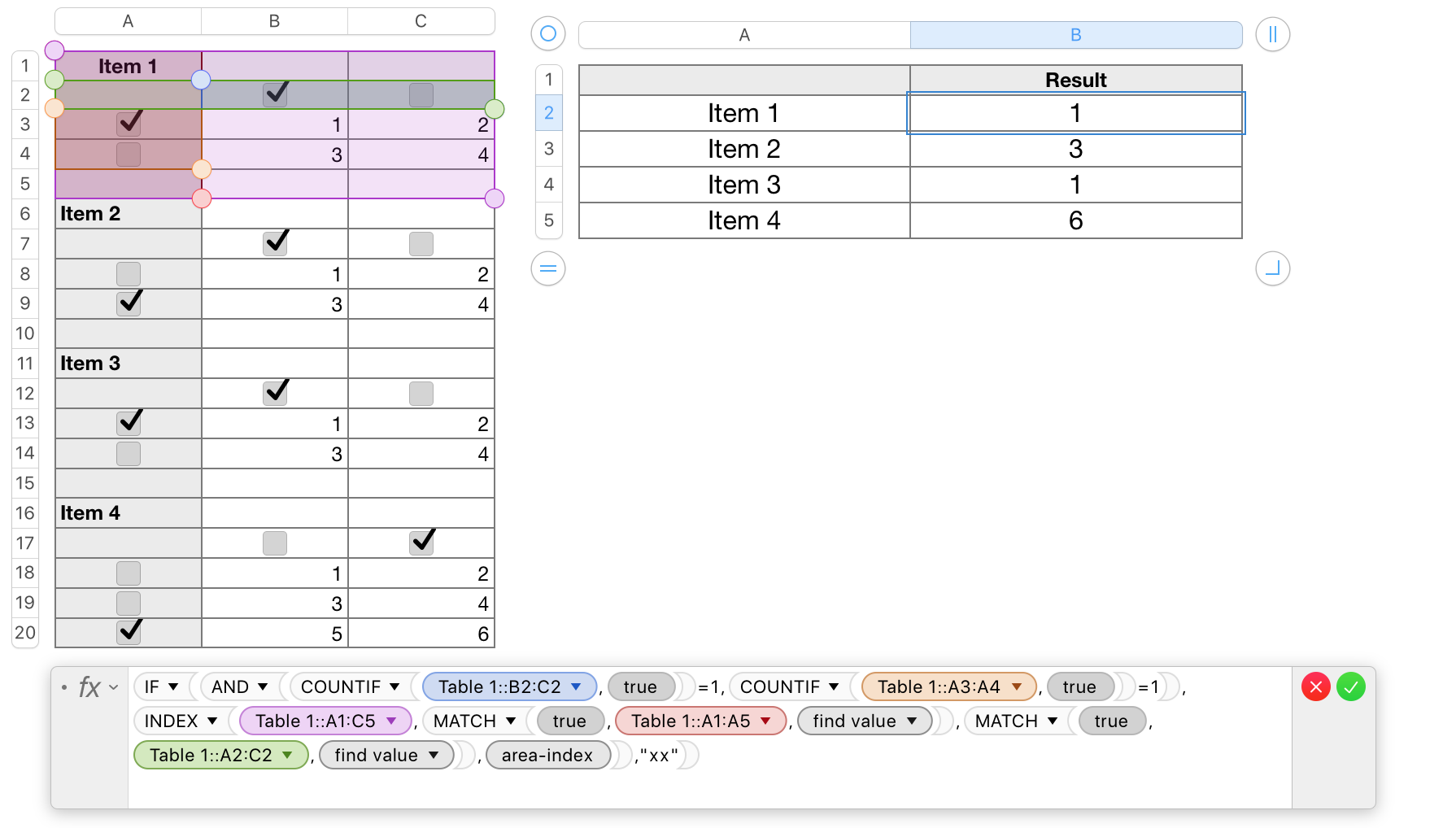
Formula in B2 of Table 2:

IF(AND(COUNTIF(Table 1::B2:C2,TRUE)=1,COUNTIF(Table 1::A3:A4,TRUE)=1),INDEX(Table 1::A1:C5,MATCH(TRUE,Table 1::A1:A5,0),MATCH(TRUE,Table 1::A2:C2,0),area-index),"xx")

As it should appear in B5 (after editing)

IF(AND(COUNTIF(Table 1::B17:C17,TRUE)=1,COUNTIF(Table 1::A18:A20,TRUE)=1),INDEX(Table 1::A16:C20,MATCH(TRUE,Table 1::A16:A20,0),MATCH(TRUE,Table 1::A17:C17,0)),"xx")

Note: "area-index" is an optional argument to index, and is not needed in this case. If you remove it, remember to aslo remove the comma immediately before it.

Regards,

Barry

Continuing:

The first line of the formula counts the number of checked boxes in column A and the number of checked boxes in Row 2. If both count results are 1, AND returns True, and IF does the MATCH and INDEX calculations to locate the correct cell an return the value in that cell.

IF either COUNTIF returns a count of zero checked cells or more than one checked cell, AND returns false, and IF returns the text message seen above.

With one cell checked in row 2 and one cell checked in column A. the formula returns the value from the cell at the intersection of the checked column and row.

The parts:

IF(expression,if-true,if-false)

expression: any test that will return only true or false

IF(AND(COUNTIF(Table 1::2:2,TRUE)=1,COUNTIF(Table 1::A,TRUE)=1),

Checked boxes contain the value TRUE, unchecked boxes contain the value FALSE. The first COUNTIF here is set to count the TRUE values in row 2, the second COUNTIF is set to count the TRUE values in column A. Each count is compared with the value 1. AND will return TRUE only if both counts return TRUE.

if-true

INDEX(Table 1::A1:D5,MATCH(TRUE,Table 1::A,0),MATCH(TRUE,Table 1::2:2,0)),

The first MATCH looks for TRUE (a checked box) in column A and returns the position in the column of the first one it finds. The second MATCH looks for TRUE in row 2, and returns the position in the row of the first one it finds.

INDEX receives those two numbers as the row-index and ˆc=column-index of the cell from which to return the contents.

if-false

"Check ONE box in Row 2 and ONE box in column A")

If expression has returned false, IF places this text value in the cell containing the formula.

Regards,

Barry

When you are having trouble getting a formula to work then it can help to reduce it down to its basics and get it working. Then add error checking and other "bells and whistles" later only if you need them.

As Barry recommends, you should consider splittingd your big table up into smaller tables (In Numbers that's easy; just select the cells you want in a separate table and drag them onto the canvas).

Then one of the tables and the formula that looks up a value from it would look like this:

=INDEX(Table 1::A$1:D$5,MATCH(TRUE,Table 1::A,0),MATCH(TRUE,Table 1::$1:$1,0))

This will show an error unless you have checked a box in the Header Column and in the Header Row. If you are still getting an error after checking boxes, then click the red warning triangle and look at the error message. If it still complains about a syntax error, then it's possible that your region expects ; in the formula instead of , . That would be the case if your region uses , as a decimal separator.

Note that this solution finds the first pair of checked boxes (first one in the column and first one in the row). So make sure you don't check too many.

SG

HI d,

IF expects a single expression in the first position, an action in the second, and an action in the third.

The expression must return a single boolean value: true, or false.

Your expression is a range of cells, some containing true, others containing false. The range will not return either of those values. Numbers will take a 'best guess' at what is expected, and return a result reflecting that choice. My test suggests that Numbers guesses you want the SUM of the values in those four cells, recognizes the values as 'text', not Boolean values, and assigns numerical value of zero to all four (this is the value assigned to any text value in a list in the SUM function) and returns the sum, 0.

To get the result for each row in your table, you need to use a single instance of IF in each row, referencing that row's individual cell in column A. Here's an example:

Column B in the example contains the formula A3 in cell B3. When that formula is filled down the column to B6, the number (row) part of the cell reference increments to match the row containing that copy of the formula. The formula copies the contents of the cell on the same row of column A, displaying it as text.

The formula shown below the table is the IF formula shown as text in the header label of column C, where "3" in A3 is represented by "n" for number. Each copy reads ONE cell in column A, gets its value (true or false), then returns the text 'checked' or 'no' depending on that value.

Column D contains the set of values shown in column B of your example. Column E contains the IF formula you need for the results you expect in your column C.

In E3: IF(A3,D3,"no")

IF gets the value from A3. If it is TRUE, IF returns the value from D3, If it is FALSE, IF returns the text value "no"

Filled down to D6, each copy of the formula references the cells in its row of Column A and Column D.

Note the lack of $ in the cell references. The Absolute Reference Operator ( $ ),

placed in front of the letter part of a cell address keeps the reference on that column as the formula is filled right or left into new columns.

Placed before the number part of a cell reference, the operator keeps the reference on that row as the formula is filled up or down into new rows.

In your case, you do not need the '$A' notation as you are not filling the formula left or right, and you do not want the $3 notation as you want each copy to refer to the 'next' row as you fill the formula down a column.

Regards,

Barry

Makes sense.

For this situation, one of the LOOKUP functions is useful. The core formula in D7, using VLOOKUP would be this one:

D7: VLOOKUP(TRUE,A:B,2,FALSE)

This formula would do the job, provided the user checks only a single box in the set.

VLOOKUP searches from the bottom of the search column, and returns the value from the first row in which it finds the search value. With this formula, Example 1 would display the red error triangle, flagging a 'can't find' error message, Examples 2 and 3 would both show "Disk size" in D7, and example 4 would show "Computer type."

To make all examples show correct results, I've added an IF statement that counts the number of checked cells, and presents the "check one box" message if the count is not 1 and the desired result if only one of the boxes is checked. The resulting formula is shown below the sample tables, and is copied below, ready to copy and paste into a table matching the ones above.

D7: IF(COUNTIF(A,TRUE)≠1,"Check one box",VLOOKUP(TRUE,A:B,2,FALSE))

Regards,

Barry

"Note that this solution finds the first pair of checked boxes (first one in the column and first one in the row). So make sure you don't check too many."

…and that, of course is the reason for adding the 'bells and whistles' wrapper to the working formula to warn you that you've checked too many (or too few).

Regards,

Barry

"But does it mean that Its not possible to show the result for all options in one cell?"

Not necessarily, but for a definitive answer, I'd need a detailed description of hat you mean by "show the result for all options in one cell."

What are the options? What would be shown in the 'one cell' for each combination of options chosen?

Regards,

Barry

Here is one way.

Details below (clicked reply too early, and won't have time to write the description before edit period ends.)

B

"could you please share your test file?"

Sorry, I don't maintain any online storage/sharing accounts where I'd be able to do that.

Regards,

Barry