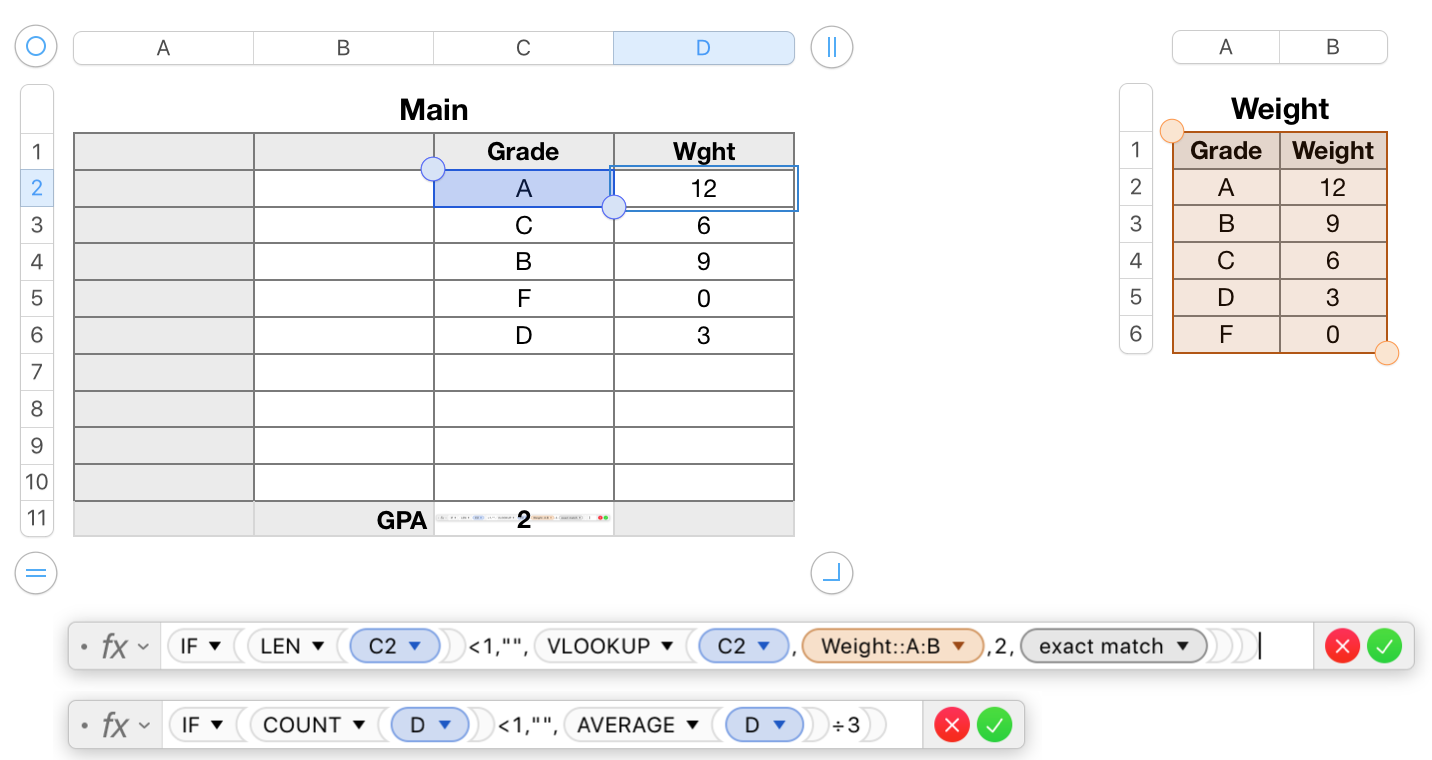
You need a lookup table to list each letter grade and its numeric equivalent.
You can then retrieve the number value for column B of your main table using VLOOKUP to find the grade letter and return the number value from the same row of the lookup table.

"Weight" is the lookup table, containing the data shown. This table contains no formulas.
"Main" is the table on which the letter grades are entered in column C.
Main contains two formulas.
The first,
IF(LEN(C2)<1,"",VLOOKUP(C2,Weight::A:B,2,FALSE))
has two parts. The core formula, shown in bold,gets the value in 'this row' of column C, searches for it in the first column of the lookup table, and returns the number value iin the second column (specified by the 2 in the formula) of the row in which it finds tha search value. he last argument (Exact Match, tells the function to accept only an exact match between'the search value and the value found.
The core formula is wrapped in an IF statment whose purpose is to prevent Nubers calling on the VLOOKUP part until there is an entry in C2
The formula is filled down from C2 to the last Body row in the table. (row 10)
The second formula:
IF(COUNT(D)<1,"",AVERAGE(D)÷3)
also has two parts.
The core formula, shown in bold, calculates the average of the grade weights returned to body cells in column D by the first formula, then divides the result by 3 to determine the GPA.
The rest is another switch, preventing the calculation until at least one weightvalue has been placed in column D by the formula in that column.
Row 1 of each table is a Header Row.
Row 11 of Main is a Footer row.
In Main, the use of a header row and footer row permits the 'letter only' reference to column D in the AVERAGE function.
Regards,
Barry