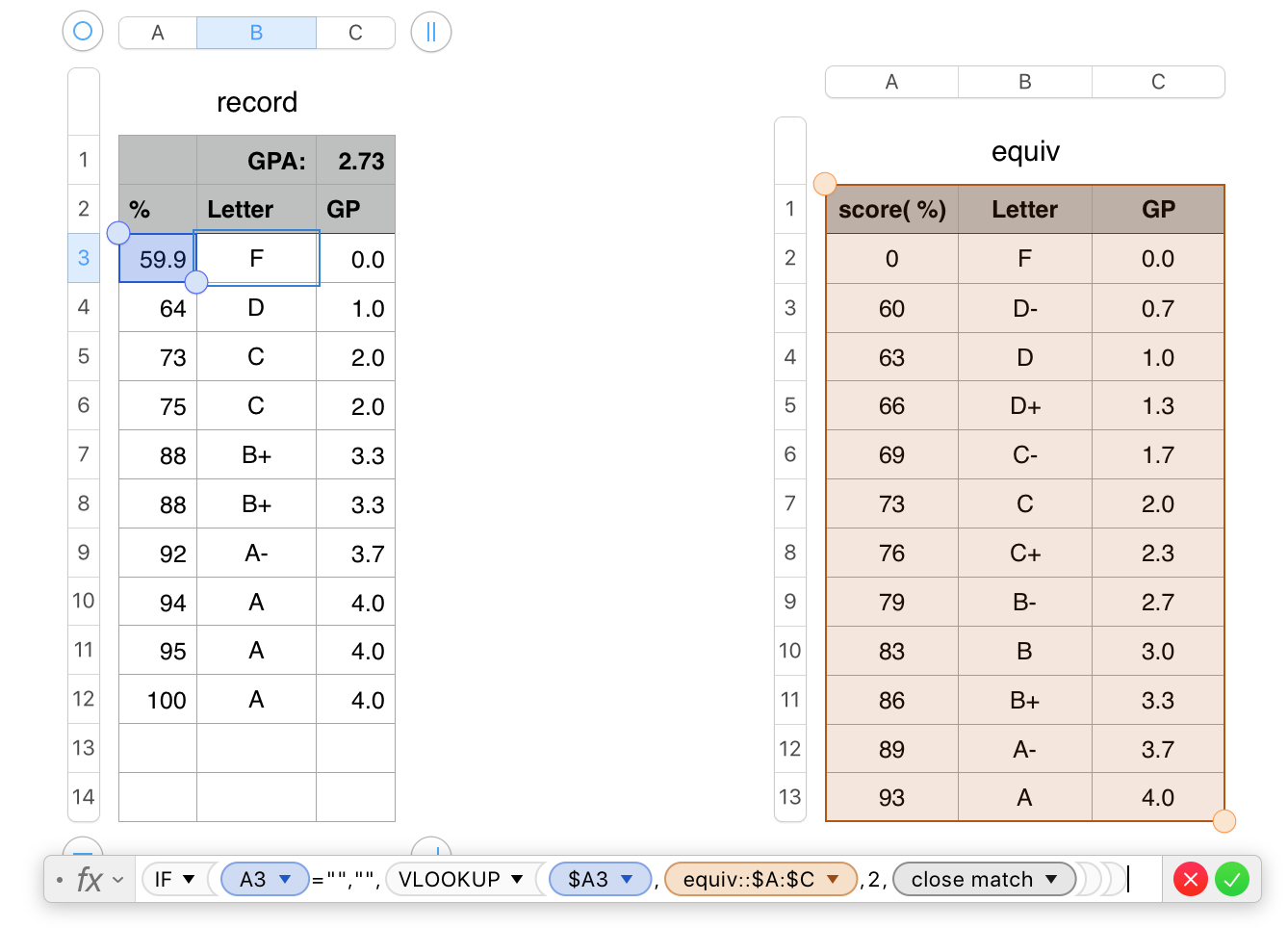
Place the values you have listed into a lookup table. Thi is the table named "equiv" on the right in the image below.
In column B, list the available letter grades from lowest to highest.
In column A list the minimum percentage score to achieve each letter grade.
In column C, list the GP score matching each letter grade,
In the Record table on the left, click in cell A1 and press option-up arrow to add a second header row above the existing one in the table.
In Row 1, leave A1 empty, enter the label "GPA: " min B1, and leave C1 empty for now.
In row 2, entr the labels shown.

Column A is used for entering a series of percentage scores.
The formula shown below the table is entered in B3 of Record.
The same formula is entered in C3, then edited to change the 2 before "close match" to a 3.
Both formulas are filled down to row 14 of theie respective columns.
If you want to calculate and display the GPA of the entered scores, enter the formula below. marked "C1" in cell C1 of this table.
C1: IF(COUNT(C)<1,"",AVERAGE(C))
B3, and filled down: IF(A3="","",VLOOKUP($A3,equiv::$A:$C,2TRUE))
C3, and filled down: IF(A3="","",VLOOKUP($A3,equiv::$A:$C,3,TRUE))
If is used in each formula to suppress Average or VLOOKUP from performing their calculations until there is at least one value in the GP column cells, or until there is an entry in 'this row' of column A.
Regards,
Barry