Line chart to only include cells with numbers

You can select just the data points you want in the chart. Create the chart with one or more data points. Edit Data References and command-click on additional data points, skipping over the ones you don't want. Removing data points is more difficult so be careful you do not accidentally select one you don't want. You can remove points by editing the data values for the series (in the sidebar when the chart is selected). You can also remove them using Edit Data References and moving/joining/resizing ranges so the point is no longer included then reselecting any points that got uncovered.

Keep the table as is, but change the data reference celsl for the chart to include only the columns which already have values entered. Edit the data references each time you enter new data.

OR

Keep the table as is, and set the data reference cells for the chart to include all the columns which currently have entered values plus those that will have values entered later.

The first option will give you a chart that you can manually expand to fit the available data each time more data becomes available.

The second will give you a chart that will initially have an abundance of 'empty' space, into which the chart can expand as more data is added to the table.

In either case, data missing from a cell will cause a gap in the line displaying the change in that datum over time.

Selecting individual data points, as shown in Badunit's post above should bypass that issue, but I think it might also reduce the two choices here to the first option only, considering the difficulty of removing chosen data points.

Regards,

Barry

An alternative method that is more automatic but also more complex:

It uses the ability of a chart to ignore hidden cells. So if your blank cells are in hidden rows, they will not be part of the chart.

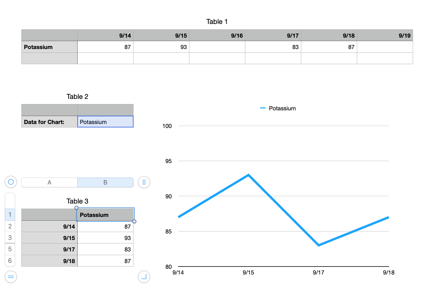
Table 2 is typed in. No formulas. The word needs to match the name in Table 1 that you want to chart.

Table 3 is made up of formulas and is filtered. As you can see it has hidden rows and is only showing the data to be charted. Make the table with as many or more rows as Table 1 has columns.

B1 =Table 2::B2

A2 =INDEX(Table 1::$1:$1,ROW())

B2 =VALUE(VLOOKUP($B$1,Table 1::$1:$3,ROW(),0)&"")

Edit that formula in B2 so it includes all rows of your table 1. I only have $1:$3.

Fill down to complete the columns

You will have error triangles at the bottom of the table if it is longer than Table 1 is wide

You will have error triangles in column B wherever there was a blank cell in Table 1.

Create your chart from this table. Use the entire table for the chart, error triangles and all.

Create a filter for the table of "show rows where column B text is not..." and type in any non-numeric text, like a space character. The table should shrink up to just the rows with data. The chart should include only those rows.

Move Table 3 to another sheet to get it out of the way. You should never have to mess with it again unless you need to add more rows to it.

Note that the formula in column B is designed around how VLOOKUP and other referencing functions will translate a blank cell into a zero. If you attach a &"" to the end, it does not do that but it makes the result text. VALUE turns it back to a number or, if it cannot, it creates an error. The filter is using that error to filter out the row.

You can control the range of cells to be included in a line chart, but Numbers will always include all columns in that range. Any empty dats cells will cause a break in the line tracking that data.

To close the gap in the chart, yo need to close the gap in the data.

Regards,

Barry

Can you post a screenshot of your data or something like, together with chart, it so we can visualize better what you are trying to do?

SG