Numbers not importing IFERROR Formula

I created an Excel spreadsheet that used that exact formula, copy/pasted from your post. I named a range Chattanooga_State. The formula worked in Excel. I imported it into Numbers 10.3.9 and it worked properly. I then went back to Excel and mangled the name Chattanooga_State so the MATCH function would be an error. When imported into Numbers it gave the "unsupported function" message when importing.

Are you sure this formula was working properly in Excel? With IFERROR wrapped around it, it is not easy to tell because it catches that error and gives you a zero instead of an error. I am thinking this import problem is really a problem with the original spreadsheet.

One additional thought: you might consider replacing the zero with "Not Found".

It appears the Excel named range 'Chattanooga_State" is Mileage!E5:E31 in Excel. It would be Mileage::Table 1::E5:E31 in Numbers. The formula is looking down column E for the point of origin and across row 3 for the destination and returning the number (miles) at the intersection of the found row and column.

=IFERROR(INDEX(Mileage::Table 1:: G5:AG31,MATCH(Calculation Sheet::Table 1::C7, Mileage::Table 1::E5:E31 ,0),MATCH(Calculation Sheet::Table 1::D7,Mileage::Table 1::G3:AG3,0)),0)

The first non-Numbers artifact I see is the "!" used in Excel to separate the worksheet name from the cell range in Excel.

The single quotes enclosing 'Chattanooga_State' are not needed in Numbers, nor is the underscore connecting the two words unless the underscore is used in the name itself.

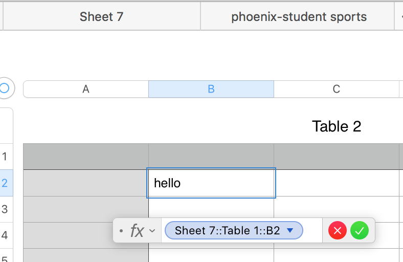
In Numbers, the full address of a cell is Sheetname::Tablename::celladdress

If the cell (or range) in on the same table as the formula, only the celladdress is needed.

If the referenced cell is on a different table from the formula,

AND the name of the other table is distinct from the named on all other tables in the document,

Numbers needs Tablename::celladdress

If the referenced cell is on a different table than the formula

AND the name of that table is the same as any other tablename in the document,

Numbers needs the full Sheetname::Tablename::celladdress

Example:

The syntax for INDEX, MATCH and IFERROR is quite similar in Numbers and Excel

Numbers will provide you with that syntax in the Function Browser article for the specific function,

And will provide you with hints in the Formula Editor if you type the first few letters of the function name then choose the function from the suggestions provided.

Here's a Numbers formula written to do essentially the same lookup function as the Excel formula provided. All tables in the example are on the same sheet, but because each has a name distinct from all others in the document, the formula would not change if the two tables were on different sheets.

Register::A is a range reference to all of column A of that table (as shown by the highlighting in the cells in the table. Ditto for Register::D.

$A$1&" "&ROW()-1 constructs a text value (Baseball 1 in the selected cell) used as a search value by MATCH,

find value is the same instruction as 0 in the Excel version.

Regards,

Barry

Recommend stripping out all the fancy formatting (merged cells, etc) and starting with simple "Numbers style" tables with a Header Row at the top. Get the formulas working and only then add formatting, if you want.

You don't show the actual formula in your screenshot but the formula you posted in your original post cannot be correct.

What are the errors you see when you click the warning triangles? They should give a clue.

SG

I am curious why you are getting the unsupported formula message in the first place. Is the formula you posted the exact formula copy/pasted from the Excel spreadsheet? If it is, the only thing I see odd is Chattanooga_State in the first MATCH. It is not the usual format for a range reference, unless it is a named reference in Excel. But named references import.

What version of Numbers are you running? INDEX and MATCH have been around forever. I can't recall if IFERROR was included from the beginning or is a more recent addition, though "recent" was still a long time ago.

Maybe it is not figuring out the named reference, which then creates a syntax error, which makes the formula unsupported. I would try to assist on reworking your formula for Numbers but I do not know what sheet, table, or range of cells is "Chattanooga_State". I believe it will have imported your tables with the name Table 1. Unless I messed something up, the Numbers version is below but you need to fill in the one range I don't know.

=IFERROR(INDEX(Mileage::Table 1:: G5:AG31,MATCH(Calculation Sheet::Table 1::C7, ENTER_RANGE_THAT_BELONGS_HERE ,0),MATCH(Calculation Sheet::Table 1::D7,Mileage::Table 1::G3:AG3,0)),0)