As I read this, the minimum accepted pledge is $2, those pledging between $200 and $4.99 will not be listed on the PLEDGES table, and if pledges of less than $2 are permitted, those will either not be listed in the csv or will be listed, but will show 0 in all five columns.
If that is correct, there should be no need for changes in what follows.
The solution uses three tables:
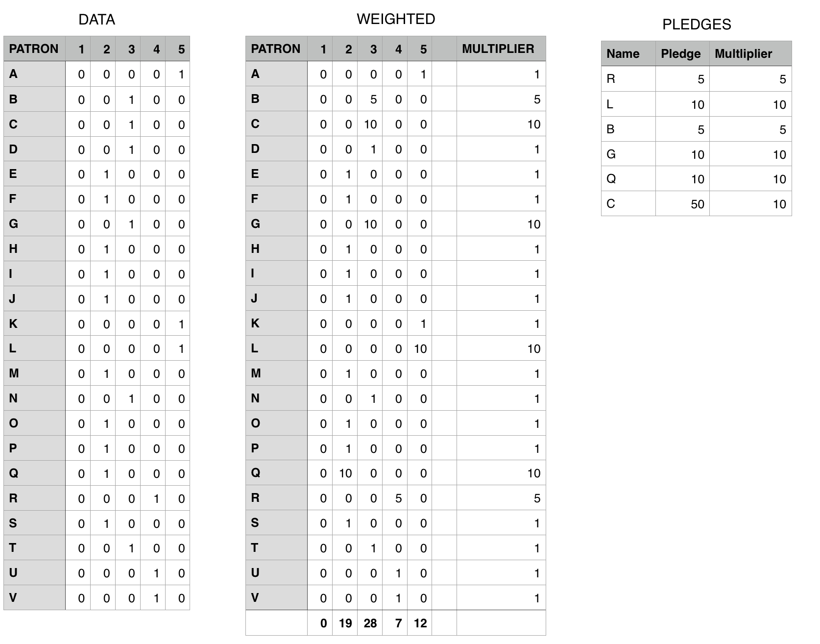
DATA is the table into which the values in the csv file will be pasted. This table contains only the pasted data shown plus the column lables in the top row.
PLEDGES is your pledge list table, with one added column to record the vote multiplier corresponding with that person's pledge.
WEIGHTED is the workhorse. All entries in this table (except the labels in row 1) are created by formula.
There are four formulas in this table:
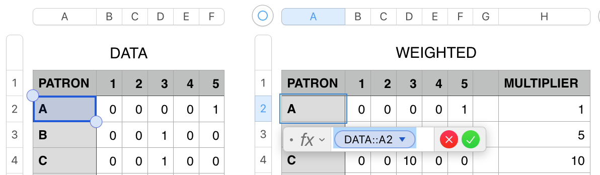
The formula in A2 is a simple cell reference to the same cell on DATA.
To enter it in A2 of WEIGHTED:
- Click once on A2, then type = to open the Formula Editor
- With the formula editor open, click once on cell A2 of DATA.
- Click the green checkmark to confirm the formula and close the editor.
Fill this formula down to the last non-footer cell in column A ( A23 ). (see Note below)
The formula in B2 collects the value from the corresponding cell of DATA and multiplies it by the value in the same row of column H of WEIGHTED.

Click on B2, open the Editor as described above, then:
- Click on cell B2 of DATA
- Type * (This will immediately change to the multiplication sign)
- Click on Cell H2 of WEIGHTED
- In the formula editor, click on the token for H2, then click the checkbox to Preserve Column.
- Click the green checkmark. to confirm the formula and close the editor.
Fill the formula right to G2, and down to row 23 (the last body row of this table)
(All cells in columns C to G of Weighted shold show zeros at this point due to th absence of numbers in column H.)
Footer row:
With the table selected, go to the Table menu and choose Footer Rows > 1 to add a Footer row to this table.
Formula in Footer Row ( C24-G24 )
In column C of the Footer row:
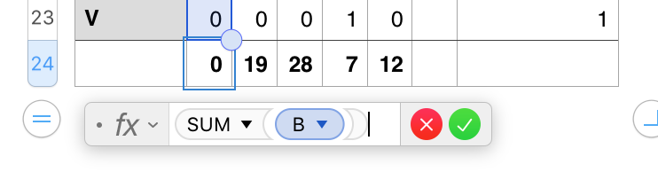
- Open the formula editor, enter the formula shown below.
- Fill right to column G.
(These results should also show zeros at this point.)
Formula in H2:
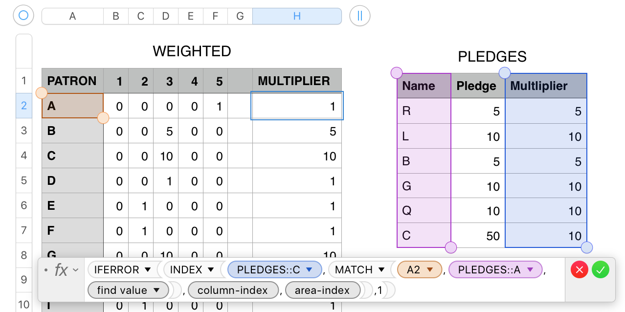
H2: IFERROR(INDEX(PLEDGES::C,MATCH(A2,PLEDGES::A,0),column-index,area-index),1)
The core formula here is a lookup formula. MATCH searches column a of PLEDGES for the name on 'this row' of WEIGHTED, and returns a number indicating the position of that name on the list.
If the name is not found, MATCH throws an error messafe, and IFERROR returns the value 1.
INDEX uses this number to locate the multiplier value in the same row of column D of PLEDGES found in A2,
Enter the formula as shown (or copy it from here and paste it into the editor for cell H2, then fill it down the rest of column H, omitting the Footer row.
NOTE on Filling a formula:
Enter the formula in to top left cell of the block into which it is to be filled.
After closing the editor, select the cell containing the formula.
Hover the mouse pointer near the edge of that cell colest to the direction in which you want to fill the formula.
Use the pointer to grab the small yellow dot that appears and drag it in the direction you want to fill,
Alternate:
After entering the formula, click the cell once to select it.
Copy.
Scrol down and right to the bottom right cell of the block into which the formula is to be filled.
Shift-click on that cell.
Press command-V.
Regards,
Barry