Unfortunately Numbers does not have an option to connect data points across a blank spot. It can be done but the only way I know of can be painful if you have more than one series on the chart. It requires splitting your table into multiple tables and making a filter that will hide blank rows. If the chart is set to not plot hidden data (which is the default), it will skip over hidden rows. This will only work for scatter charts. Your main table can stay like it is, you can create new tables that pull the data from your main table just for the chart.
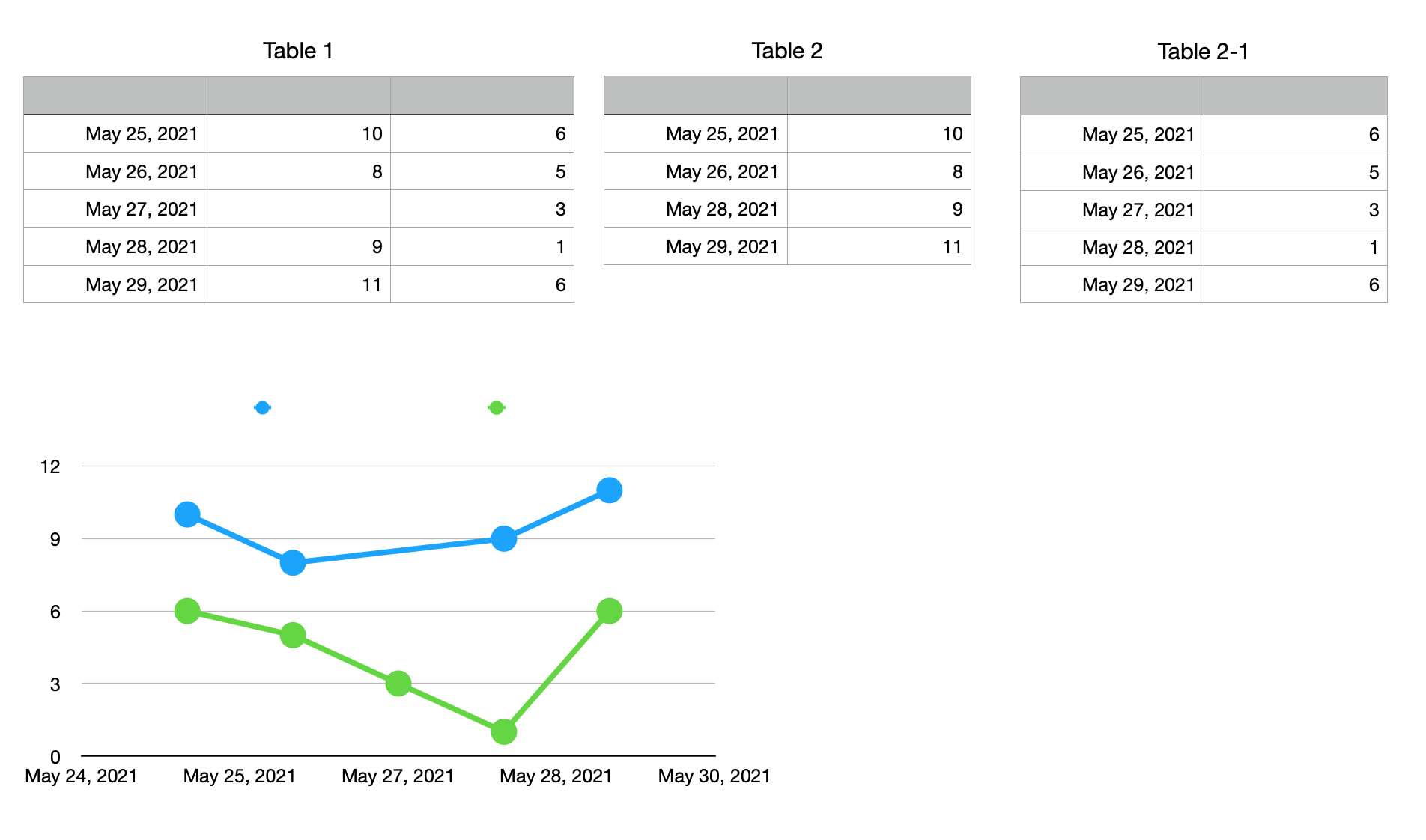
Table 1 is where the data is entered
Table 2 is for the first series. It should be as many rows as or longer than Table 1. No header columns because it will be for a scatter chart. In the screenshot it has a filter on it hiding the one "blank" row. It is actually many rows longer than Table 1.
B2 =IF(Table 1::B≠"",Table 1::A,"hide")
C2 =Table 1::B
Fill down to complete the columns
If Table 2 is longer than Table 1, you must use references like "Table1::B" in the formulas, not ones like "Table 1::B2". When you add rows to Table 1, these references will pick up the newly added rows. If Table 2 is longer than Table 1, you will have a lot of error triangles. Don't worry about them.
Create a filter on Table 2 of "show rows where column A text is not hide".
This filter will hide the rows with blank data. It also hides all the rows with error triangles
Turn the filter off for now.
Copy/Paste Table 2 to make Table 2-1
Change all references of Table 1::B to Table 1::C in the formulas.
Select both columns of Table 2 and create a scatter chart
Edit Data References and select both columns of Table 2-1 to add the second series
In the black area above column A click on the disclosure triangle and deselect "share X values"
Turn on the filters on the two tables.
You can cut/paste the two tables to another sheet, out of the way.